U.S. Department of the Interior
U.S. Geological Survey
Techniques and Methods 3
-
A19
Levels at Gaging Stations
Chapter 19 of
Section A, Surface-Water Techniques
Book 3, Applications of Hydraulics
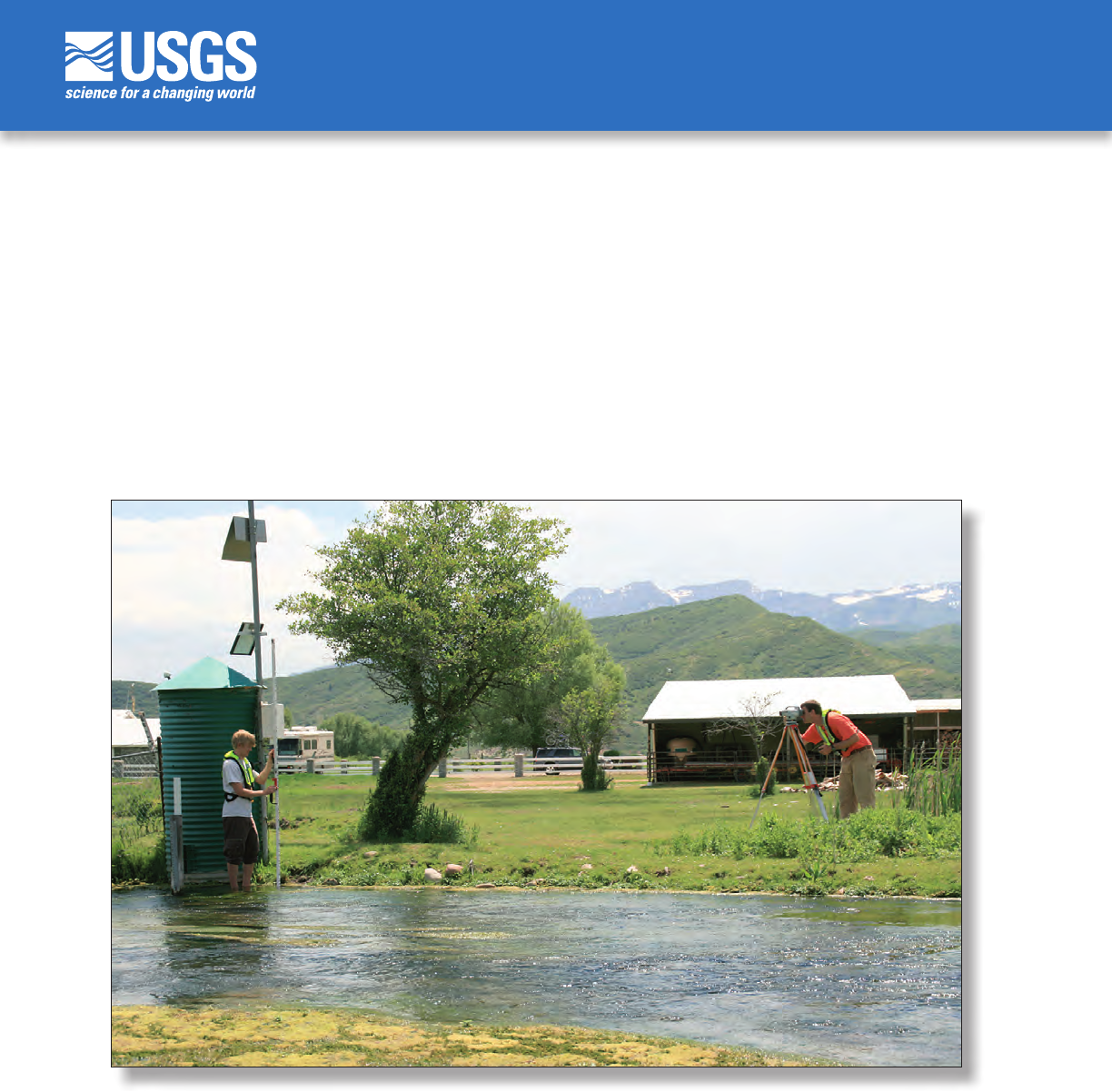
Cover: View of levels being run at U.S. Geological Survey streamflow-gaging
station 10156000, Snake Creek near Charleston, Utah.
Photograph taken by K. Michael Nolan, U.S. Geological Survey, June 30, 2010.
Back Cover: USGS topographic field party, circa 1925, with a Wye level on a
tripod and two stadia rods. Photograph by U.S. Geological Survey.
Levels at Gaging Stations
By Terry A. Kenney
Chapter 19 of
Section A, Surface-Water Techniques
Book 3, Applications of Hydraulics
Techniques and Methods 3–A19
U.S. Department of the Interior
U.S. Geological Survey
U.S. Department of the Interior
KEN SALAZAR, Secretary
U.S. Geological Survey
Marcia K. McNutt, Director
U.S. Geological Survey, Reston, Virginia: 2010
For more information on the USGS—the Federal source for science about the Earth, its natural and living resources,
natural hazards, and the environment, visit http://www.usgs.gov or call 1-888-ASK-USGS
For an overview of USGS information products, including maps, imagery, and publications,
visit http://www.usgs.gov/pubprod
To order this and other USGS information products, visit http://store.usgs.gov
Any use of trade, product, or firm names is for descriptive purposes only and does not imply endorsement by the
U.S. Government.
Although this report is in the public domain, permission must be secured from the individual copyright owners to
reproduce any copyrighted materials contained within this report.
Suggested citation:
Kenney, T.A., 2010, Levels at gaging stations: U.S. Geological Survey Techniques and Methods 3-A19, 60 p.

iii
Preface
This series of manuals on techniques and methods (TM) describes approved scientific and data-
collection procedures and standard methods for planning and executing studies and laboratory
analyses. The material is grouped under major subject headings called “books” and further
subdivided into sections and chapters. Section A of book 3 is on surface-water techniques.
The unit of publication, the chapter, is limited to a narrow field of subject matter. These
publications are subject to revision because of experience in use or because of advancement
in knowledge, techniques, or equipment, and this format permits flexibility in revision and
publication as the need arises. Chapter A19 of book 3 (TM 3–A19) deals with levels at gaging
stations. The original version of this chapter was published in 1990 as U.S. Geological Survey
(USGS) Techniques of Water-Resources Investigations, chapter A19 of book 3. New and
improved equipment, as well as some procedural changes, have resulted in this revised second
edition of “Levels at gaging stations.”
This edition supersedes USGS Techniques of Water-Resources Investigations 3A–19, 1990,
“Levels at streamflow gaging stations,” by E.J. Kennedy.
This revised second edition of “Levels at gaging stations” is published on the World Wide Web
at http://pubs.usgs.gov/tm/tm3A19/ and is for sale by the U.S. Geological Survey, Science
Information Delivery, Box 25286, Federal Center, Denver, CO 80225.
iv
This page intentionally left blank.
v
Contents
Preface ...........................................................................................................................................................iii
Abstract ...........................................................................................................................................................1
Introduction.....................................................................................................................................................1
Purpose and Scope .......................................................................................................................................1
Differential Leveling and Leveling Equipment ..........................................................................................2
Level Instruments..................................................................................................................................2
Optical Levels ...............................................................................................................................3
Electronic Digital Levels .............................................................................................................3
Parallax ..........................................................................................................................................4
Checking the Engineer’s Level ...........................................................................................................4
Fixed-Scale Test ..........................................................................................................................6
Peg Test .........................................................................................................................................6
Manufacturer-Recommended Collimation Test ......................................................................7
Collimation Error and Balanced Sightline Distances .....................................................................8
Leveling Rods.........................................................................................................................................9
Inspection of Leveling rod .......................................................................................................10
Proper Care and Use of a Rod Level .......................................................................................11
Correcting for Rod Scale Expansion or Contraction Due to Temperature Variations ....11
Considerations for Secondary Devices Used for Vertical Measurements ......................13
Establishment of Gage Datum ...................................................................................................................13
Installation of Reference Marks .......................................................................................................14
Referencing a Gage Datum to an Established Datum ..................................................................16
Frequency of Gaging-Station Levels ........................................................................................................17
Preparation for Running Levels .................................................................................................................18
Determining the Need for Levels .....................................................................................................18
Compiling Historic Level Notes and Site Sketch Maps ................................................................19
Considerations for Site Conditions ..................................................................................................19
Running Levels ............................................................................................................................................19
Standards and Requirements for Gaging-Station Levels ....................................................20
Circuit-Closure Error ................................................................................................................20
Assessing a Level Circuit and Adjusting Elevations .....................................................................25
Methods for Taking Foresights on Gages and the Water Surface .............................................27
Vertical Staff Gage ....................................................................................................................27
Electric Tape Gage .....................................................................................................................27
Wire-Weight Gage .....................................................................................................................30
Crest-Stage Gage ......................................................................................................................32
Inclined Staff Gage ....................................................................................................................33
Water Surface ............................................................................................................................36
Resetting Gages Based on the Results of Levels ..........................................................................36
Methods for Simplifying Complex Level Circuits ...........................................................................36
Separating Complex Level Circuits into a Set of Sequentially Closed Simple
Level Circuits ................................................................................................................37
vi
Running Levels—Continued
......................................................................................................................19
Methods for Simplifying Complex Level Circuits—Continued ....................................................36
Using a Suspended Weighted Steel Tape to Carry Elevation to or from a Bridge
Structure .......................................................................................................................39
Bridge-Down Method .....................................................................................................44
Ground-Up Method ..........................................................................................................44
Office Procedures .......................................................................................................................................45
Applying Datum Corrections to Gage Height Time Series ..........................................................45
Developing a Site-Specific Historical Level Summary .................................................................45
Developing a Site Sketch Map .........................................................................................................45
Auxiliary Data to be Obtained During Level Runs ..................................................................................46
Summary........................................................................................................................................................46
References Cited..........................................................................................................................................46
Glossary .........................................................................................................................................................49
Appendix A. Fixed-Scale Test Form .......................................................................................................51
Appendix B. Peg Test Form ....................................................................................................................53
Appendix C. Level Notes Form ...............................................................................................................55
Appendix D. Historical Level Summary Form ......................................................................................57
Appendix E. Summary of Selected Requirements and Tolerances for Gaging Station Levels ....59
Contents—Continued
Figures
Figure 1. Diagram of differential leveling using an engineer’s level and leveling rods ……… 2
Figure 2. Photographs of optical levels …………………………………………………… 3
Figure 3. Photographs of electronic digital levels ………………………………………… 4
Figure 4. Photographs of bar-code leveling rods …………………………………………… 5
Figure 5. Diagram of an engineer’s level and rod scales set up for the fixed-scale test …… 7
Figure 6. Diagram of an engineer’s level and leveling rods set up for the two-peg test …… 7
Figure 7. Photographs of self-reading leveling rods ………………………………………… 10
Figure 8. Scale of a self-reading Philadelphia rod ………………………………………… 11
Figure 9. Photographs of stand-alone and permanently attached rod levels ……………… 12
Figure 10. Photograph of a steel tape with 1 pound of tension ……………………………… 13
Figure 11. Diagram of gage datum at a station ……………………………………………… 14
Figure 12. Typical reference marks ………………………………………………………… 15
Figure 13. Extreme depth of frost map ……………………………………………………… 16
Figure 14. Decision tree for determining if levels are needed ……………………………… 17
Figure 15. Complete set of level notes for a level circuit with two instrument setups ……… 21
Figure 16. Complete set of level notes for a level circuit with eight instrument setups ……… 23
Figure 17. Photographs of foresights being taken on staff plates by holding leveling rods
on nails driven into backing boards ……………………………………………… 28
Figure 18. Picture of an electric tape gage with a pocket rod held on a stack of coins at
the elevation of the index ………………………………………………………… 29
Figure 19. Photographs of a wire-weight gages mounted on bridges ……………………… 31

vii
Conversion Factors
Multiply By To obtain
Length
inch (in.) 2.54 centimeter (cm)
foot (ft) 0.3048 meter (m)
Temperature in degrees Fahrenheit (°F) may be converted to degrees Celsius (°C) as follows:
°C = (°F - 32)/1.8
Figure 20. Photograph of a cantilevered wire-weight gage located to the left of a
stilling well ………………………………………………………………………… 32
Figure 21. Stage-related wire-weight corrections determined from levels ………………… 33
Figure 22. Photograph of a crest-stage gage where the index is the bottom cap …………… 34
Figure 23. Photograph of a crest-stage gage where the index is a bolt installed through
the pipe …………………………………………………………………………… 35
Figure 24. Photograph of an inclined staff gage installed on a streambank ………………… 35
Figure 25. Leveling diagram showing objective points in a complex circuit and level notes
for a complex leveling circuit …………………………………………………… 37
Figure 26. Leveling diagram and level notes showing 3 simple level circuits used to
replace 1 complex level circuit …………………………………………………… 39
Figure 27. Leveling diagram and level notes illustrating the use of a suspended steel tape
to carry elevations from a bridge down to a streamside gage location and from
a streamside gage location up to a bridge ……………………………………… 41
Figures—Continued
Tables
Table 1. Notes for gaging station levels run when all sightline distances are equal and
the instrument used has a collimation error of 0.01 foot per 100 feet …………… 9
Table 2. Notes for gaging station levels run when sightline distances between the
instrument and objects vary in the same order for two setups and the
instrument used has a collimation error of 0.01 foot per 100 feet ………………… 10
Table 3. Notes for gaging station levels run when sightline distances between the
instrument and objects vary inversely for two setups and the instrument used
has a collimation error of 0.01 foot per 100 feet …………………………………… 11
Table 4. Approximate coefficients of thermal expansion for common leveling rod-scale
materials ………………………………………………………………………… 15
Table 5. Requirements for demonstrating gaging station stability ………………………… 21
Table 6. Example summary of levels where the stability criterion is not met ……………… 21
Table 7. Standards and select requirements for leveling ………………………………… 28
Table 8. Standards and adopted requirements for gaging station levels ………………… 28
Table 9. Computed adjustment values for each instrument setup of a four-instrument
level circuit with a closure error of –0.005 foot …………………………………… 30
Table 10. Technique for rounding off numbers ……………………………………………… 30
viii
This page intentionally left blank.

Abstract
Operational procedures at U.S. Geological Survey gaging
stations include periodic leveling checks to ensure that gages
are accurately set to the established gage datum. Differential
leveling techniques are used to determine elevations for
reference marks, reference points, all gages, and the water
surface. The techniques presented in this manual provide
guidance on instruments and methods that ensure gaging-
station levels are run to both a high precision and accuracy.
Levels are run at gaging stations whenever differences in gage
readings are unresolved, stations may have been damaged, or
according to a pre-determined frequency. Engineer’s levels,
both optical levels and electronic digital levels, are commonly
used for gaging-station levels. Collimation tests should be
run at least once a week for any week that levels are run, and
the absolute value of the collimation error cannot exceed
0.003 foot/100 feet (ft).
An acceptable set of gaging-station levels consists of a
minimum of two foresights, each from a different instrument
height, taken on at least two independent reference marks, all
reference points, all gages, and the water surface. The initial
instrument height is determined from another independent
reference mark, known as the origin, or base reference mark.
The absolute value of the closure error of a leveling circuit
must be less than or equal to
0.003 n
ft, where n is the total
number of instrument setups, and may not exceed |0.015| ft
regardless of the number of instrument setups. Closure error
for a leveling circuit is distributed by instrument setup and
adjusted elevations are determined. Side shots in a level
circuit are assessed by examining the differences between the
adjusted rst and second elevations for each objective point
in the circuit. The absolute value of these differences must be
less than or equal to 0.005 ft. Final elevations for objective
points are determined by averaging the valid adjusted rst and
second elevations. If nal elevations indicate that the reference
gage is off by |0.015| ft or more, it must be reset.
Introduction
At gaging stations where water-surface elevation or
stage is measured, the U.S. Geological Survey (USGS) sets
gages to read the stage above a specied reference surface
called the gage datum (Kennedy, 1990). Equipment in most
gaging stations measures and records stage at a frequency
of 15 minutes. At streamow gaging stations, discrete
measurements of streamow, made by hydrographers, are
paired with a representative stage value. Over time, these
pairings dene a site-specic stage-discharge relation to
which recorded stage values are applied to obtain a continuous
streamow record. To provide accurate and relevant data, it is
imperative that gages agree with the established gage datum
for the life of the station. To check and ensure that gages are
properly set to gage datum, differential leveling techniques are
used. Levels are run at gaging stations according to a standard
set of frequency requirements, when unresolved gage reading
differences have been identied, or when the station has been
damaged.
Purpose and Scope
The purpose of this manual is to document the
procedures that should be followed when running levels
to check that gages are set to the established gage datum.
Leveling equipment is discussed, along with specic precision
requirements, desired accuracy, and calibration requirements.
The required frequency for running gaging-station levels is
outlined and presented in an easy to follow decision tree. The
procedure for running levels at gaging stations is described
in detail and illustrated in example level circuits. Specic
error tolerances for both circuit closure and objective-point
elevation differences are presented. Methods for taking
foresights to various types of gages are discussed, and nally,
ofce procedures associated with gaging-station levels are
outlined. This manual describes new procedures for running
levels at gaging stations that supersede those described by the
previous USGS Techniques of Water-Resources Investigations
Report “Levels at Streamow Gaging Stations” by E.J.
Kennedy (1990).
Levels at Gaging Stations
By Terry A. Kenney
2 Levels at Gaging Stations
Differential Leveling and Leveling
Equipment
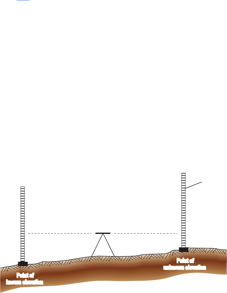
Differential leveling is the process of measuring the
vertical difference between a point of unknown elevation and
a point of known elevation (McCormac, 1983). By measuring
this difference, an elevation can be determined for the point
of unknown elevation. At gaging stations, this measurement
is most commonly made using an engineer’s level and a
calibrated leveling rod (g. 1). The engineer’s level is set up
about equidistant from the point of known elevation and the
point(s) of unknown elevation. A shot from the engineer’s
level is rst made to a leveling rod that is held on the known
elevation point. This reading on the leveling rod is called
a backsight (BS). The BS, which is the vertical distance of
the engineer’s level above this point, is added to the known
elevation of that point to determine the elevation of the
engineer’s level, or the height of the instrument. Shots are then
made from the engineer’s level to the leveling rod that is held
on point(s) of unknown elevation. These readings are called
foresights. A foresight (FS) is the distance of the engineer’s
level above the point and is subtracted from the instrument
height to determine elevation.
Differential leveling techniques are used at gaging
stations to determine elevations for reference marks, reference
points, gages, and the water surface. Reference marks are
objects (for example, brass tablets, steel rods, or bolts) that
are installed in the most stable locations near the gage and
are used to adjust the gages as necessary to keep them in
agreement with the gage datum (Kennedy, 1990). Reference
points are objects (for example, bolts, nails, or screws) that
are installed in locations to facilitate the determination of
gage heights by measuring their distance from the water
surface. A variety of engineer’s levels and leveling rods can be
used to run levels at streamow-gaging stations. The USGS
reports stage at most gaging stations in increments of 0.01 ft.
Therefore, gaging-station levels, which are used to verify
that gages agree with the gage datum, must be measured at
a higher level of precision and accuracy. Precision describes
the closeness of one measurement to another while accuracy
describes how close a given measurement is to the true value
(McCormac, 1983). The precision required of gaging-station
levels is 0.001 ft, while the desired accuracy is less than
0.010 ft. Instruments selected for running levels at gaging
stations must be capable of meeting these precision and
accuracy requirements.
Level Instruments
Many surveying instruments are available that have
several different equipment options and can perform
a variety of surveying tasks. Levels at gaging stations
require measurements of vertical distance and do not need
measurements of horizontal distance or horizontal angle.
Engineer’s levels are the most common instruments used for
running levels at gaging stations. Most engineer’s levels meet
the desired accuracy of less than 0.010 ft and the required
precision of 0.001 ft for gaging-station levels. Surveying
technology is continually changing, and other types of
surveying instruments, such as tilting instruments, may be
capable of meeting these accuracy and precision standards.
Point of
known elevation
Point of
unknown elevation
BS
BS Backsight
FS Foresight
FS
Leveling rod
Instrument
IP021599_Figure 1. Schematic of differential leveling.
EXPLANATION
Figure 1. Differential leveling using an engineer’s level and leveling rods.
Differential Leveling and Leveling Equipment 3
The techniques and methods presented in this manual provide
guidance on using engineer’s levels that ensures gaging-station
levels are run to a high level of precision and accuracy. Before
other types of surveying instruments are used for running
gaging-station levels, techniques and methods specic to those
instruments that ensure precision and accuracy requirements
are met must be rigorously documented. Engineer’s levels,
which are sometimes referred to as line or spirit levels, can
be classied in two general categories: optical levels and
electronic digital levels.
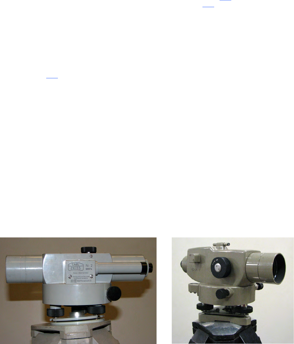
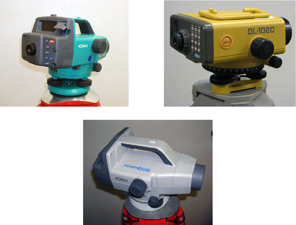
Optical Levels
Optical levels (g. 2) are used to manually read the
leveling rod that is held on an objective point. When using
an optical level, the operator reads the value off the rod at the
cross hair of the level. Self-reading rods used in gaging-station
levels are graduated to 0.01 ft. Precision requirements call
for the operator of an optical level to estimate measurements
within 0.001 ft. The ability to accurately estimate to 0.001 ft is
determined by the distance from the instrument to the rod, the
magnication power of the level’s optics, and environmental
conditions, such as the presence of heat waves. In general, the
magnication of optical levels is about 30 times and allows
readings as precise as 0.001 ft up to a distance of about 150 ft.
Most modern optical levels are automatic, or self-leveling
— the instrument levels itself precisely after being leveled
manually with its circular (bull’s eye) level (Kennedy, 1990).
Many older optical levels, such as the Dumpy level, are not
self-leveling and are time-consuming to set up and level.
These older instruments are also easily knocked out of level,
which can introduce unquantied errors into the leveling
circuit.
Electronic Digital Levels
Electronic digital levels (g. 3) automatically read a
bar-code leveling rod (g. 4) held on an objective point.
When using an electronic digital level, the operator sights in
the bar-code leveling rod using the optical view nder and
then interrogates the instrument to make a measurement. The
instrument then shows the value on its digital display screen.
Many electronic digital levels are equipped with logging
and computational functions that can be used when running
levels. Electronic digital levels contain optical systems that
also allow the level to be used manually. Like optical levels,
distances to objective points and environmental conditions
can limit the utility of electronic digital levels. Electronic
digital levels provide some distinct advantages over optical
levels; for example, because the instrument automatically
reads the leveling rod, any subjectivity in manually estimating
the measurement to 0.001 ft is removed. Similarly, the
potential for misreading the leveling rod is eliminated when
using electronic digital levels. When using data-logging
features common to many electronic digital levels, errors
associated with manually transcribing measurements can
also be eliminated. A disadvantage of electronic digital levels
is that the electronic nature of these instruments introduces
the potential for system failures to occur while in the eld.
Fortunately, the optical capability serves as a backup to the
electronic system. It is common when running levels at gaging
stations to use a secondary device, such as a steel tape, to
take shots on objects located in places where a rod cannot
be placed. Further, FSs to some objects (such as wire-weight
gages) are made by sighting in the object at the cross hair of
the instrument. Digital systems, which require a bar-code rod,
cannot be used for such shots. For these reasons, both the
optical and the digital systems of electronic digital levels must
be maintained and tested frequently.
Figure 2. Optical levels.
4 Levels at Gaging Stations
Figure 3. Electronic digital levels.
Parallax
A sharply focused level is important for accurate readings
of the leveling rod. A properly focused instrument locates the
graduations of the leveling rod at the plane of the cross hairs.
Parallax is the relative movement of the image of the leveling
rod with respect to the cross hairs as the observer’s eye moves.
This is caused by the objective lens not being focused on the
leveling rod (Kennedy, 1990). To check for parallax, slightly
move your eye up and down while sighting in a leveling rod. If
the rod appears to move with respect to the cross hair, parallax
is present. Parallax usually can be eliminated by adjusting the
objective focus. Diligence in refocusing the instrument for all
readings and checking for parallax will eliminate erroneous
measurements associated with improper focus.
Checking the Engineer’s Level
An engineer’s level is set up to measure the vertical
distance from objective points to the level plane of the
instrument. When applying the techniques of differential
leveling, a properly leveled instrument is assumed to be on a
horizontal plane at the determined elevation of the instrument
or instrument height. Collimation error is a measurement of
the inclination of a level’s line of sight (Breed and others,
1970; McCormac, 1983; Kennedy, 1990), or the deviation
from the horizontal plane. Collimation error is reported as
a vertical deviation over a set distance, such as 0.xxx ft per
100 ft. If horizontal distances from the instrument to each
object that a FS or BS is taken on are known, collimation
corrections can be computed and applied. However, levels
at gaging stations do not require measurements of horizontal
distance, and therefore, the collimation error of the instrument
is preserved in all measurements and is not corrected for.
Differential Leveling and Leveling Equipment 5
A
B
IP021599_Figure 4. Rods
Figure 4. Bar-code leveling rods. A. separated multi-section rod
showing the self-reading rod scale on the second side.
Collimation error of an engineer’s level is determined by
running a xed-scale test, a two-peg test, or another accepted
collimation test. These tests check how true the instrument
is sighting on a horizontal plane. Given the precision with
which gaging-station levels are run (0.001 ft) and the criteria
that determine a valid level run at a gaging station (these are
outlined in detail in the section on “Assessing a Level Circuit
and Adjusted Elevation”), the tolerance for the collimation
error of an instrument cannot exceed the absolute value (| |)
of 0.003 ft/100 ft. Instruments possessing collimation errors
greater than |0.003| ft/100 ft should be adjusted by qualied
personnel or by a certied facility. Following any adjustments
made to an instrument, a collimation test must be performed
and documented to verify that the instrument was adjusted
correctly.
The criteria for an acceptable level run include a limit
on circuit-closure error and a maximum difference between
the rst and second elevations of any objective point in the
level circuit. Conditions exist that can cause an instrument
with a collimation error greater than |0.003| ft/100 ft to yield
results that meet the criteria for an acceptable level circuit and
yet still produce nal elevations that are incorrect because of
the collimation error (see section on “Collimation Error and
Balanced Sightline Distances”). In order to minimize errors
associated with instrument calibration, a collimation test
(xed-scale, peg, or other accepted test) must be performed
and documented at least once per week (National Oceanic
and Atmospheric Administration, 1981; Federal Geodetic
Control Committee, 1984) for each week that gaging-station

6 Levels at Gaging Stations
levels are run. There should not be more than 7 days between
a collimation test and a set of levels. If a level is found to
have a collimation error greater than |0.003| ft/100 ft, all
gaging- station levels run since the previous collimation
test must be discarded and re-run. For this reason, it is
recommended to run collimation tests more frequently. When
electronic digital levels are used, these tests should be done for
both the optical and digital systems.
Fixed-Scale Test
A xed-scale test uses two mounted rod scales set to
the same datum and spaced about 120 ft apart to determine
the collimation error of an instrument (g. 5). A xed-scale
test can be set up outdoors between trees, deeply set posts,
or buildings at a reasonably level location, or can be set up
indoors; for example, between columns or doorframes in a
long corridor of a large building (Kennedy, 1990). To install
the scales, place the instrument equidistant from the mounting
locations. Install each scale such that the readings from the
level to each scale are equal. To test the collimation of the
level, set it up as close as possible to one scale. Read each
scale from this location, and measure the horizontal distances
to each scale. The length of d
2
should not exceed 110 ft to
avoid curvature and refraction effects. Horizontal distances
can be determined using the stadia hairs of the level, the
distance reported by an electronic digital level, or a measuring
tape. From these readings, the collimation error can be
computed using the equation (Kennedy, 1990):
1 2
2 1
1
2
( )
100* ,
( )
where
is the collimation error, in unit length
per 100 unit lengths,
is the reading obtained from the near
rod scale, in unit length,
is the reading obtained from the far
R R
c
d d
c
R
R
−
=
−
1
2
rod scale, in unit length,
is the distance to the near rod scale,
in unit length, and
is the distance to the far rod scale, in
unit length, which should be less
than 110 ft.
d
d
(1)
If the absolute value of the collimation error is greater than
0.003 ft/100 ft, the level must be adjusted. A diagram of a
xed-scale test showing the variables of equation 1 is shown
in gure 5. A xed-scale test form is provided in appendix A.
Peg Test
A peg test does not require scales to be mounted and
can be run with the instrument and rod in any reasonably
level location. Several versions of peg tests are used. The
one described here, commonly referred to as a two-peg test,
was adapted from the USGS Geography Discipline, formerly
known as the USGS Survey and National Mapping Division
(Kennedy, 1990). Two pegs or marks should be established
and spaced about 120 ft apart (g. 6). The instrument is set up
as close as possible to one of the pegs. Shots are taken to the
rod held on the near peg and the far peg. Distances from the
instrument to the pegs are measured, using the stadia hairs,
the digital system, or a measuring tape. The instrument is then
moved as near as possible to the other peg, and again shots
are taken to each and distances are measured. From these
measurements the collimation error can be computed using the
equation (Kennedy, 1990):
1 3 2 4
2 4 1 3
1
2
( ) ( )
100* ,
( ) ( )
where
is the collimation error, in unit length
per 100 unit lengths,
is the reading taken on the near peg
from the first instrument setup,
in unit length,
R R R R
c
d d d d
c
R
R
+ − +
=
+ − +
3
4
is the reading taken on the far peg
from the first instrument setup,
in unit length,
is the reading taken on the near peg
from the second instrument
setup, in unit length,
is the reading taken on th
R
R
1
2
e far peg
from the second instrument setup,
in unit length,
is the distance to the near peg
from the first instrument setup,
in unit length,
is the distance to the far peg from
the first instrument
d
d
3
4
setup, in unit
length,
is the distance to the near peg from
the second instrument setup, in
unit length, and
is the distance to the far peg from the
second instrument setup, in unit
length.
d
d
(2)
Differential Leveling and Leveling Equipment 7
The average of d
2
and d
4
should be less than 110 ft to avoid
curvature and refraction effects. If the absolute value of the
collimation error is greater than 0.003 ft/100 ft, the instrument
must be adjusted. A diagram of a peg test showing the
variables of equation 2 is shown in gure 6. A peg test form
is provided in appendix B and is also contained in the Gaging
Stations Level Notes form (appendix C).
Manufacturer-Recommended Collimation Test
Some manufacturers of level instruments provide
a recommended method for testing and adjusting for
collimation error. Some of the electronic digital levels
contain preprogrammed tests and adjustment routines
that provide for efcient and convenient collimation
checks. Some preprogrammed checks may require the
instrument to be located a specied distance from the rod.
If manufacturer- recommended methods meet the 0.001-ft
precision and the less than 0.010-ft accuracy requirements for
gaging-station levels and report collimation error as a vertical
deviation over a specied distance, they can be used as the
weekly collimation test. Weekly tests are required for both the
optical and digital systems of the electronic instruments.
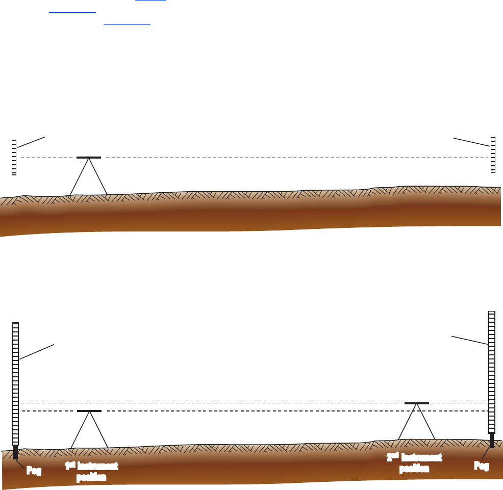
Figure 5. Engineer’s level and rod scales set up for the fixed-scale test. R, the reading obtained from a rod scale; d, the distance
to a rod scale. Modified from Kennedy (1990).
R
1
R
2
d
1
d
2
IP021599_Figure 5. Schematic of fixed scale test.
Fixed scale
Fixed scale
Instrument
Figure 6. Engineer’s level and leveling rods set up for the two-peg test. R, the reading obtained from a leveling rod; d, the
distance to a peg. Modified from Kennedy (1990).
R
1
R
3
R
2
R
4
d
1
d
2
d
3
d
4
IP021599_Figure 6. Schematic of peg test.
1 Instrument
position
st
2 Instrument
position
nd
Leveling rod
Leveling rod
Peg
Peg
8 Levels at Gaging Stations
Collimation Error and Balanced Sightline
Distances
Collimation error is a measure of the inclination of a
level’s line of sight. Unless corrected using measurements of
horizontal distance, this systematic error is preserved in all
measurements made with the level. Balancing the sightline
distances to all objects to which shots are taken minimizes
the effects of collimation error on nal elevations. However,
balancing sightline distances in a gaging-station level circuit
is often not feasible. Under ideal conditions when sightline
distances are perfectly balanced, collimation error preserved
in FSs and BSs does not affect the nal computed elevations.
An example is an instrument that has a high collimation error
of 0.010 ft/100 ft and sightline distances that equal 100 ft
(table 1). Each BS and FS shows an error of 0.010 ft, because
the instrument has a collimation error of 0.010 ft/100 ft and
the distances are all 100 ft. Even though each shot contains
collimation error, because the horizontal distances are equal,
the error in each shot is equal. The collimation error indicates
that the line of sight of the level is angled downwards causing
readings of the leveling rod to be 0.010 ft low. Because the
errors are equal for each shot, the true differences in elevation
between the objective points can be accurately determined, and
therefore, the nal elevations of the objective points are the
true elevations and the circuit-closure error is 0.000 ft. If this
were a level circuit, ideally the level would not be used because
the absolute value of the collimation error is greater than
|0.003| ft; however, because the sightline distances are perfectly
balanced, the collimation error does not adversely affect
the nal elevations because the true differences in elevation
between the objective points are determined in this circuit.
Collimation error begins to have a profound effect
on nal elevations when sightline distances are extremely
unbalanced. However, the effect of collimation error can be
masked when the distances between the instrument and the
objective points remain the same for the second instrument
setup. Table 2 provides an example of how the effects of
collimation error can go unnoticed. This example uses the
same level circuit as the previous example, but sightline
distances range from 10 to 200 ft. In this circuit, the distance
to each of the objects remained the same for the second
instrument setup. Errors contained in each BS and FS ranged
from 0.001 to 0.020 ft. In a real gaging-station level circuit,
these errors would not be known because horizontal distances
are not measured. The two elevations acquired for each
objective point differ from the true elevations, yet the closure
error is 0.000 ft. In this example circuit, an instrument with
a large unknown collimation error was used, and unless a
comparison was made with the historical elevations, one
would assume that the level circuit met the criteria for a
valid level circuit of closure error and the difference between
adjusted rst and second objective point elevations (discussed
in detail below). This introduces the potential for gages to be
set or adjusted incorrectly during a level run.
The sightline distances should be inverted in order to
reveal collimation errors in a circuit consisting of unbalanced
sightline distances, which, as shown above, can produce
erroneous nal elevations. In the previous example with
unbalanced sightline distances, the second instrument setup
was located in the same position as the rst instrument setup.
The level circuit appeared to be valid, as evidenced by a
closure error of 0.000 ft and no differences between rst
and second elevations for each objective point, yet the nal
Object
Distance
from
instrument
to object
BS
error
1
BS HI
FS
error
1
FS Elevation
Closure
error
1st and 2nd
elevation
differences
True
elevations
Difference
from true
elevation
RM1 (origin) 100 0.010 5.260 105.260 0.010 NA
2
100.000 NA NA 100.000 NA
RM2 100 NA NA NA 0.010 7.121 98.139 NA NA 98.139 0
RM3 100 NA NA NA 0.010 2.042 103.218 NA NA 103.218 0
TP 100 NA NA NA 0.010 3.343 101.917 NA NA 101.917 0
Instrument moved and re-leveled
TP 100 0.010 4.343 106.260 0.010 NA 101.917 NA NA 101.917 0
RM3 100 NA NA NA 0.010 3.042 103.218 NA 0 103.218 0
RM2 100 NA NA NA 0.010 8.121 98.139 NA 0 98.139 0
RM1 100 NA NA NA 0.010 6.260 100.000 0.000 NA 100.000 0
Table 1. Notes for gaging station levels run when all sightline distances are equal and the instrument used has a collimation error of
0.01 foot per 100 feet.
[All values are given in feet. Elevations are referenced to an arbitrary gage datum. BS, backsight; HI, height of instrument; FS, foresight; RM, reference mark;
TP, turning point; NA, not applicable]
1
Computed from the collimation error and the distance from the instrument to the object.
2
Given elevation in the level circuit.
Differential Leveling and Leveling Equipment 9
Object
Distance
from
instrument
to object
BS
error
1
BS HI
FS
error
1
FS Elevation
Closure
error
1st and 2nd
elevation
differences
True
elevation
Difference
from true
elevation
RM1 (origin) 10 0.001 5.251 105.251 0.001 NA
2
100.000 NA NA 100.000 NA
RM2 100 NA NA NA 0.010 7.121 98.130 NA NA 98.139 –0.009
RM3 150 NA NA NA 0.015 2.047 103.204 NA NA 103.218 –0.014
TP 200 NA NA NA 0.020 3.353 101.898 NA NA 101.917 –0.019
Instrument moved and re-leveled
TP 200 0.020 4.353 106.251 0.020 NA 101.898 NA NA 101.917 –0.019
RM3 150 NA NA NA 0.015 3.047 103.204 NA 0.000 103.218 –0.014
RM2 100 NA NA NA 0.010 8.121 98.130 NA 0.000 98.139 –0.009
RM1 10 NA NA NA 0.001 6.251 100.000 0.000 NA 100.000 0.000
Table 2. Notes for gaging station levels run when sightline distances between the instrument and objects vary in the same order for
two setups and the instrument used has a collimation error of 0.01 foot per 100 feet.
[All values are given in feet. Elevations are referenced to an arbitrary gage datum. Distances from the instrument to each object remained the same after the
instrument was moved. BS, backsight; HI, height of instrument; FS, foresight; RM, reference mark; TP, turning point; NA, not applicable]
1
Computed from the collimation error and the distance from the instrument to the object.
2
Given elevation in the level circuit.
elevations were incorrect, because the FS errors caused by
the collimation error of the instrument were equal for the two
shots taken to each objective point.
Table 3 shows an example of the same level circuit
run with an instrument with the same collimation error of
0.010 ft/100 ft, but with the sightline-distances inverted so that
the object farthest from the initial instrument setup is closest
to the instrument for the second setup. The range of error
contained in the FSs and BSs associated with the collimation
error of the instrument is similar to those in the previous
example because the same distances were used. Again, these
errors would not be known because the horizontal distances
are not measured when levels are run at gaging stations. By
inverting the sightline distances a signicant closure error
is revealed. If this example were an actual level circuit and
the instrument had a large (unknown) collimation error,
the sightline distances were unbalanced, but the sightline
distances were inverted for the second instrument setup, the
closure error criterion for a valid level circuit would have
indicated a problem with the circuit. By inverting the sightline
distances in a circuit that has unbalanced sightline distances,
unknown collimation errors of an instrument can be reected
in the closure error. If the location of objective points and
the locations for setting up the instrument cause unbalanced
sightline distances to be unavoidable, it is recommended that
these distances be inverted so that the object that was farthest
from the rst instrument setup becomes closest to the second
instrument setup. The technique of inverting the sightline
distances is designed to expose any unknown instrument error
in the circuit closure error, thus alerting the user of possible
systematic instrument error.
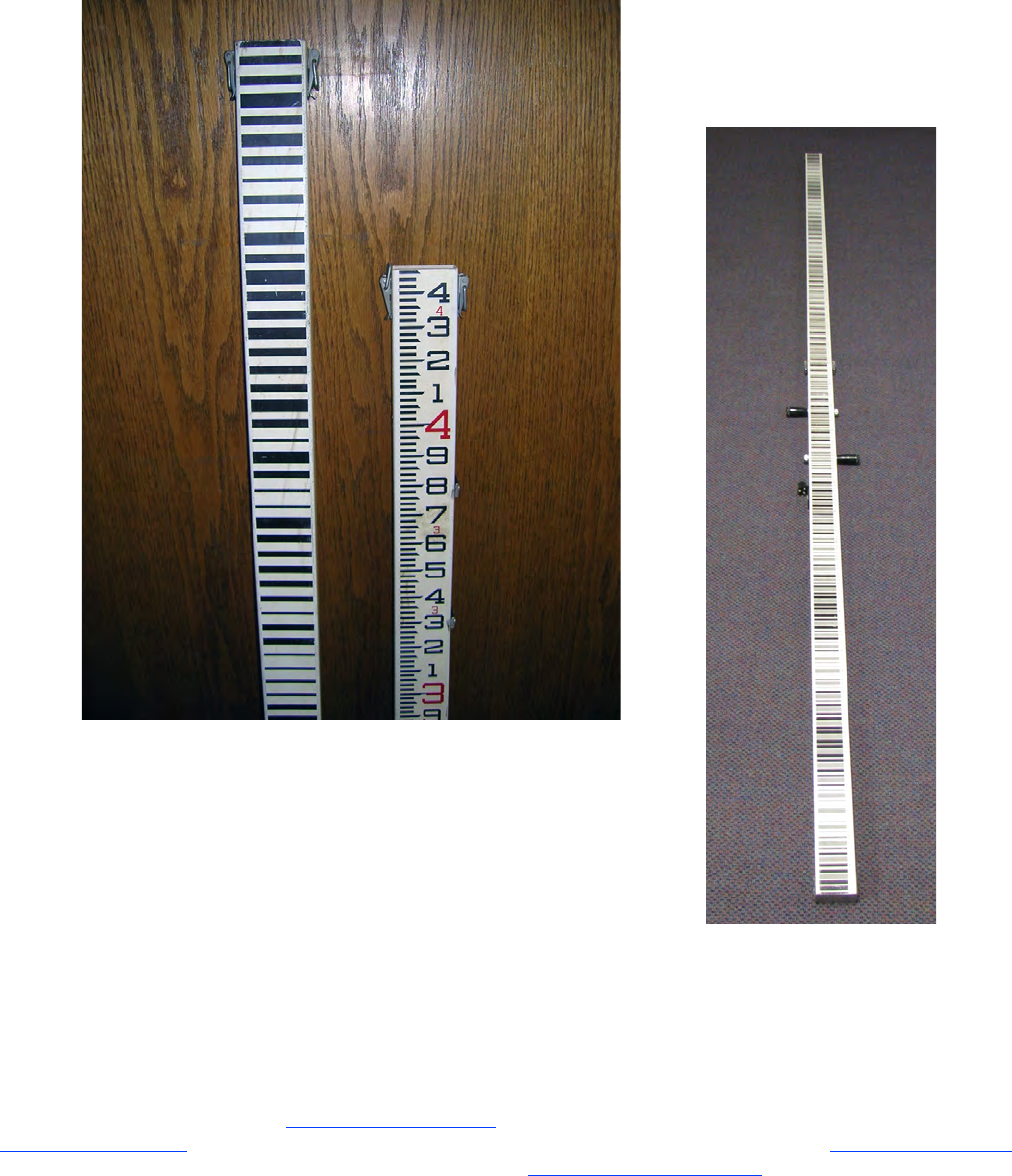
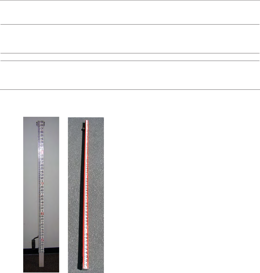
Leveling Rods
Many kinds of leveling rods are available for use in
running levels at gaging stations. Rods come in different
lengths, many are expandable, and they are made of different
materials. Many rods, such as the “Philadelphia” or “Chicago”
style rods, are made of a structural material, often wood or
berglass, and a rod-scale material, such as Invar or steel.
Invar is a nickel steel alloy, commonly used for precise
measuring equipment and has a very low coefcient of thermal
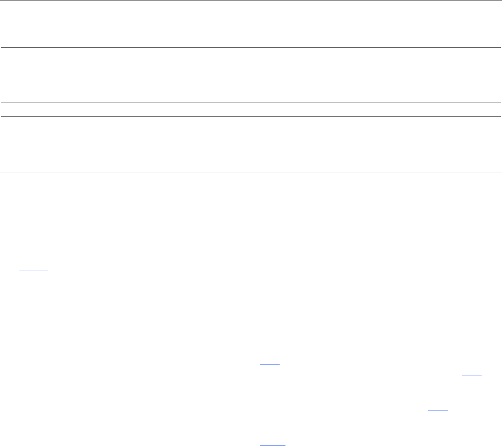
expansion (CTE). Self- reading rods with numeric scales
(g. 7) are used with optical engineer’s levels, while electronic
digital levels use leveling rods with bar-code scales (g. 4).
The scales of self-reading rods are typically divided into feet
and tenths and hundredths of feet by means of alternating
black and white spaces (McCormac, 1983) (g. 8). Bar-code
leveling rods often have a self-reading scale on the second
side of the rod to use with the optical system of the instrument
(g. 4A). For gaging-station levels, self-reading rods must
be graduated to 0.01 ft and readings are visually interpolated
in order to meet the measurement-precision requirement of
0.001 ft. Regardless of the type of engineer’s level, when
running levels at gaging stations, it is good practice to not
extend a rod more than about 16 ft because of the difculty
in holding a tall rod steady and level on an objective point. A
leveling rod should always be used in conjunction with a rod
level.
10 Levels at Gaging Stations
Inspection of Leveling rod
Leveling rods should be examined regularly to ensure
that their scales are set correctly and that their structure,
specically the bottom surface, is free of damage or debris. If
a leveling rod is found to be damaged it should be removed
from service. Thermal expansion or contraction of the material
of the rod scale should be considered when the rod is used
for gaging-station levels. The most common materials for
leveling-rod scales include Invar, berglass, steel, and wood.
Most rod scales are calibrated at the standard temperature of
68°F. The entire scale length for a self-reading rod should
be veried with an independent measuring tape from the
bottom of the rod. Similar independent verication checks of
all other measuring devices used when running levels should
also be done. All verications should be made indoors at the
standard temperature of 68°F. Rods should be checked with
a measuring tape at each foot marking along the length of the
scale and at both sides of any joints between scale sections.
If all graduations are accurate to within |0.002| ft, the rod is
satisfactory (Kennedy, 1990). If a rod scale is found to be
outside of the |0.002|-ft tolerance, adjust the scale if possible
or remove the leveling rod from service. At temperatures
greater than the calibration or standard temperature, the rod
scale will expand causing measurements to be lower than
they actually are, and at temperatures less than the calibration
temperature, contraction of the rod scale will have the opposite
effect. To minimize both errors in shots taken to leveling
rods, and the need to apply corrections to measurements due
to thermal expansion or contraction, it is recommended that
leveling rods (including all devices used as rods during level
Object
Distance
from
instrument
to object
BS
error
1
BS HI
FS
error
1
FS Elevation
Closure
error
True
elevations
Difference
from true
elevation
RM1 (origin) 200 0.020 5.270 105.270 0.020 NA
2
100.000 NA 100.000 NA
RM2 150 NA NA NA 0.015 7.126 98.144 NA 98.139 0.005
RM3 100 NA NA NA 0.010 2.042 103.228 NA 103.218 0.010
TP 10 NA NA NA 0.001 3.334 101.936 NA 101.917 0.019
Instrument moved and re-leveled
TP 200 0.020 4.353 106.289 0.020 NA 101.936 NA 101.917 0.019
RM3 150 NA NA NA 0.015 3.047 103.242 NA 103.218 0.024
RM2 100 NA NA NA 0.010 8.121 98.168 NA 98.139 0.029
RM1 10 NA NA NA 0.001 6.251 100.038 -0.038 100.000 0.038
Table 3. Notes for gaging station levels run when sightline distances between the instrument and objects vary inversely for two setups
and the instrument used has a collimation error of 0.01 foot per 100 feet.
[All values are given in feet. Elevations are referenced to an arbitrary gage datum. BS, backsight; HI, height of instrument; FS, foresight; RM, reference mark;
TP, turning point; NA, not applicable]
1
Computed from the collimation error and the distance from the instrument to the object.
2
Given elevation in the level circuit.
Figure 7. Self-reading leveling rods.

Differential Leveling and Leveling Equipment 11
runs) be used at temperatures near the calibration temperature
of the rod scale whenever possible. Determining the need
for and computing temperature corrections is discussed
in the section on “Correcting for Rod Scale Expansion or
Contraction Due to Temperature Variations.”
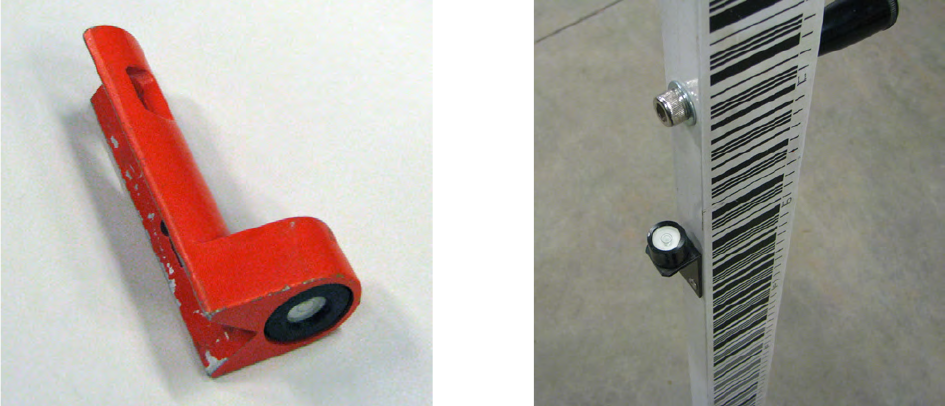
Proper Care and Use of a Rod Level
It is important that the leveling rod be held vertical
when levels are run at gaging stations. To ensure that the
leveling rod is vertical, a rod level should always be used.
Rod levels are either stand alone (g. 9A) and are used with
multiple leveling rods, or permanently attached and dedicated
to a single leveling rod (g. 9B). The stand-alone rod levels
consist of a bull’s eye bubble level mounted on a 90-degree
or square channel material. The 90-degree channel allows the
rod level to be held along the vertical axis of either a square or
round leveling rod. Rod levels should be checked for plumb
regularly and adjusted if necessary. To test the rod level, any
corner such as a wall corner that has been veried to be level
Figure 8. Scale of a self-reading Philadelphia rod.
This reading is 2.140 ft
Feet are marked by
red numbers.
Tenths of feet are
represented by
black numbers.
The x.x00 and x.x50
marks on strips are
pointed.
This reading is 2.050 ft
Small red numbers
indicate the
associated foot
sections
This reading is 2.127 ft
Foot marks are represented
with long strips
Hundredths of feet are represented
by the top and bottom of black
strips. The top of strips represent
even numbers and the bottom of
strips represent odd numbers.
IP021599_Figure 8. Reading the rod.
using a carpenter’s level can be used. Most rod levels have
screws that are used to adjust how the bubble level is seated
in its mount. When checking for plumb, the bubble should be
examined for expansion. If the bubble has expanded beyond
the circular level indicator line, the rod level should be
discarded.
Correcting for Rod Scale Expansion or
Contraction Due to Temperature Variations
At constant temperatures, measurements can be precisely
corrected for expansion and contraction of the rod-scale
material due to temperature variation. All materials have
a determined coefcient of thermal expansion (CTE), and
the CTE for the rod scale should be readily available from
the manufacturer of the rod. Material compositions of rod
scales vary, particularly for berglass rods; therefore, it is
recommended that the rod scale CTE be obtained directly
from the manufacturer. For reference, CTE ranges for some
common leveling rod-scale materials are provided in table 4.
12 Levels at Gaging Stations
The rod-scale material-specic CTE, the standard temperature,
and the rod-scale temperature at the time the leveling rod is
used for a measurement are used in the following equation to
determine the correction for expansion or contraction due to
temperature variation:
CTE * ( ),
w
here
is the correction for expansion or
contraction due to temperature
variation,in unit length,
CTE is the rod scale material specific
coefficient of thermal expansion,
in 1/ degrees Fah
t o
t
C L T T
C
= −
− −
renheit or
1/ degrees Celsius (examples
contained in table 4),
is the length of the measurement,
in unit length,
is the rod scale temperature at the
time of the measurement, in
degrees Fahrenheit or de
L
T −
grees
Celsius, and
is the standard temperature, in
degrees Fahrenheit (usually 68 F)
or degrees Celsius (usually 20 C).
o
T
°
°
(3)
The rod-scale temperature, T, can be measured directly by an
infrared thermistor, or if the rod is not in the direct sun, air
temperature can be used as a surrogate for the rod temperature.
To determine whether corrections are needed for a given level
circuit, rst compute or estimate the maximum elevation
difference between the origin reference mark and any point in
the level circuit. This is the difference between the elevation
of the origin and either the highest or the lowest point that a
FS will be taken on. Substitute this difference for L in equation
3 and compute C
t
. If the absolute value of C
t
is greater than
0.003, all FSs and BSs of the circuit should be corrected for
temperature-related expansion or contraction. Individual FSs
and BSs taken during a level run can be corrected by adding
the rod reading to the computed expansion or contraction
correction value by using the equation
corrected read read
corrected
read
(CTE* ( )),
where
is the sight (backsight or foresight)
corrected for expansion or contraction
due to temperature variation, in unit
length,
is the sight (backsight
o
S S S T T
S
S
= + −
or foresight)
obtained from the leveling rod, in
unit length,
CTE is the rod-scale material-specific
coefficient of thermal expansion, in
1/degrees Fahrenheit or 1/degrees
Celsius (examples contained in table 4),
is the rod-scale temperature at the time
of the measurement, in degrees
Fahrenheit or degrees Celsius, and
is the standard temperature, in degrees
Fahrenheit (usually 68°F) or degrees
Cel
o
T
T
sius (usually 20°C).
(4)
A
B
Figure 9. Stand-alone A. and permanently attached B. rod levels.
Establishment of Gage Datum 13
Rod-scale
material
Approximate coefficient of thermal expansion
in length/length/degree
Fahrenheit (1/°F)
in length/length/degree Celsius
(1/°C)
Invar
1
0.8 × 10
–6
1.4 × 10
–6
Wood
1
2.1 × 10
–6
to 2.8 × 10
–6
3.8 × 10
–6
to 5 × 10
–6
Steel tape
2
6.45 × 10
–6
12 × 10
–6
Fiberglass
1
17 ×10
–6
to 22 × 10
–6
30.6 ×10
–6
to 39.6 × 10
–6
Table 4. Approximate coefficients of thermal expansion for
common leveling rod-scale materials.
1
From http://www.engineeringtoolbox.com/linear-expansion-
coefcients-d_95.html.
2
From Breed, Hosmer, and Bone (1970).
Considerations for Secondary Devices Used for
Vertical Measurements
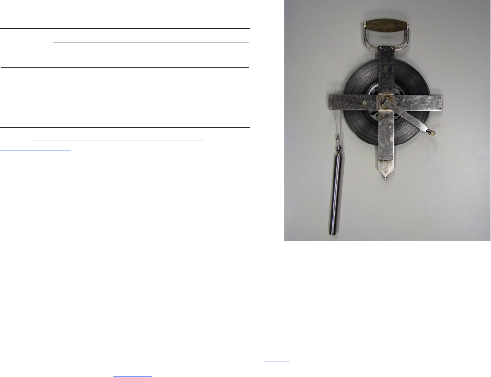
When running levels at gaging stations, a secondary
measuring device other than a leveling rod might be required
to take FSs on gages or to carry elevations over a large vertical
distance. The CTE for the materials that compose secondary
devices used in a level circuit should be obtained and used to
correct FSs and BSs when appropriate. Any secondary devices
used must meet the precision and accuracy requirements of
gaging-station levels. When using a measuring tape to carry
elevations between a bridge deck and a low water bank,
the tape should be weighted so that the tape is not stretched
and the tension applied by the weight should ensure that the
tape is suspended vertically. Figure 10 is a photograph of
a steel tape with a 1-pound weight that is commonly used
for measuring water levels in wells. This same equipment
can be used for tape-down measurements or for carrying
elevations over a large vertical distance. The practical limit of
measurement precision for this tape-down method is ±0.01 ft
(U.S. Geological Survey, 1980). If used when running levels
at gaging stations to carry elevations between a bridge deck
and a low water bank, the FSs or BSs should be estimated to
0.001 ft.
Wind can have a profound effect on suspended measuring
devices, particularly those suspended from a bridge. Wind
will cause a suspended tape to bend and articially increase
the vertical distance the tape is spanning. Wind effects cannot
be accounted for, so vertical measurements using a suspended
measuring tape affected by wind should be avoided.
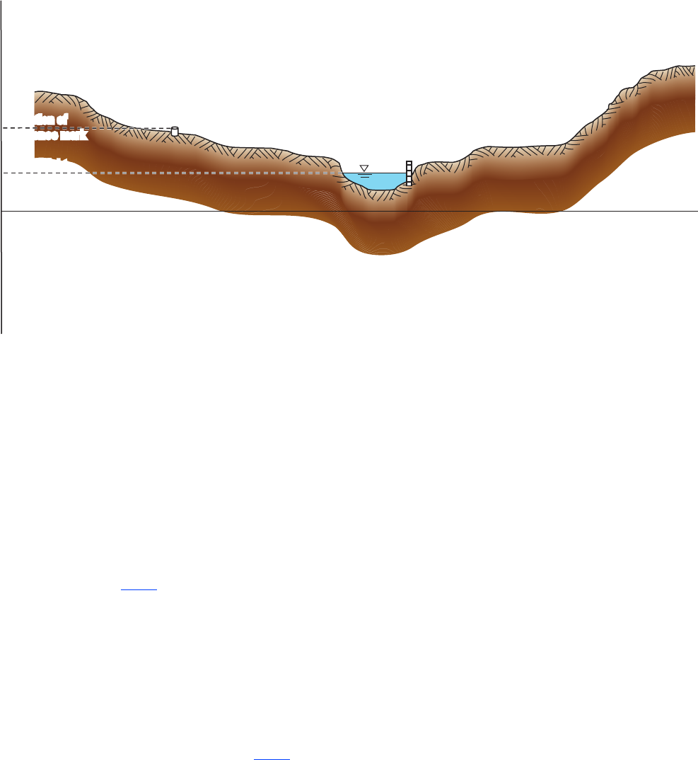
Establishment of Gage Datum
The gage datum is the reference surface at a gaging
station to which all gages are set (Corbett and others, 1943)
(g. 11). The reference surface is represented by the 0.000-ft
mark on the gages and should be located well below the
streambed, below any likely gage height of zero ow (GZF).
The gage datum is usually an arbitrary reference but it can
be tied to an established datum, such as the North American
Vertical Datum of 1988 (NAVD 88), through the use of
established benchmarks. When a gaging station is being
established where no station has existed previously, the gage
datum should be set low enough to ensure that the lowest
gage height ever likely to be recorded while the stream is
owing is at least 1 ft (Kennedy, 1990). When establishing
the gage datum, the current water depth over the hydraulic
control of the gage pool should be known and the potential
maximum streambed scour should be considered. Experience
with stream channels of similar materials, geometry, and
basin characteristics may provide some indication of the
potential magnitude of streambed scour. Because negative
gage heights are undesirable, the gage datum reference surface
that is selected should be well below the estimated maximum
scour depth to avoid negative gage heights over the life of the
station.
Figure 10. Steel tape with 1 pound of tension.
IP021599_Figure 10. Steel weight tape
14 Levels at Gaging Stations
Gage datum, 0.000 feet
Gage height
Elevation of
reference mark
ELEVATION IN GAGE DATUM
IP021599_Figure 11. Gage datum
Staff
gage
Water
surface
Reference mark
Figure 11. Gage datum at a station.
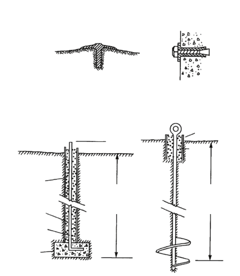
Installation of Reference Marks
Reference marks are installed and elevations are
determined in the gage datum when gaging stations are
established. Stable and permanent reference marks facilitate
maintaining that the gages at a station are set to the gage
datum over the life of the station. Typical reference marks
include gaging-station tablets cemented and drilled into rock
outcrops, bolts drilled into masonry walls, steel rods driven
and cemented into stable ground, and other earth anchors
located below frost lines (g. 12). Reference marks provide
a means for recovering the gage datum if the gaging station
is destroyed or is removed and reactivated sometime later.
The most stable locations for reference marks are often rock
outcrops and substantial masonry structures. Bridges often
provide a stable environment for reference marks; however,
bridges that sway or have a high trafc volume may not be
desirable because precise measurements are difcult to make
with a level and rod. In the absence of rock outcrops and
stable masonry structures, reference marks can be anchored at
depths below the local frost depth in stable soils (g. 13). The
methods used by the U.S. Department of Commerce, National
Oceanic and Atmospheric Administration, and National Ocean
Survey for establishing geodetic benchmarks (Floyd, 1978)
can provide guidance for installing reference marks. Clay soils
that expand and contract during seasonal variations in soil
moisture should be avoided (Kennedy, 1990).
Gaging stations should have a minimum of three
independent reference marks; more than three are
recommended whenever possible in case one (or more)
proves to be unstable or is destroyed. These marks should be
located independently of one another. For example, if one or
more reference marks are installed on a bridge structure, at
least two others should be installed somewhere away from
(and independent of) the bridge. Furthermore, reference
marks should be located independently of any gage, gage
infrastructure, or instream control structure, because reference
marks are used to track vertical changes over time to the gages
and to the other marks. If reference marks and gages are not
independent of one another, determining vertical differences
becomes difcult.
When locating reference marks, other considerations
should be made. Access to reference marks during ood
conditions is important to verify that the recorder is
accurately set to the gage datum in case the reference gage
is inaccessible. Ideally, at least one reference mark should
be located outside of the oodplain. When determining
the locations of reference marks, running levels should be
considered and, if possible, marks should be located so that
sightline distances are balanced and levels can be run in an
efcient manner. The potential for damage or destruction
of reference marks related to construction, specically road
construction or future land development, should be considered.
Finally, reference marks should be easily found from
descriptive statements in the station description document. As
discussed later, site sketches showing the location of reference
marks should be prepared. If vegetation is likely to obscure
marks over time, exact measurements from local objects
should be provided and a witness post should be installed.
Establishment of Gage Datum 15
Figure 12. Typical reference marks.
IP021599_Figure 12. Setting marks
Modified from Kennedy (1990).
Gaging-station tablet
cemented in hole drilled
in rock outcrop
3
/
8
-inch brass bolt and washer
in masonry wall
3
/
8
-in. reinforcing
steel
Steel rod in
concrete base
Earth anchor
4-inch PVC pipe
4-inch PVC pipe
lining
Concrete
base
3
-
4 inches
Below frost
line or at
a minimum
of 3 feet deep
Below frost
line or at
a minimum
of 3 feet deep
gravel
Clean gravel
16 Levels at Gaging Stations
Referencing a Gage Datum to an Established
Datum
It is desirable to reference an arbitrary gage datum to
a commonly used established datum, such as NAVD 88, at
all gaging stations. This is especially important at stations
used by the National Weather Service for ood forecasting
or at locations where ood proles are likely to be needed
(Kennedy, 1990). Generally, two methods are used to tie a
gage datum to an established datum - running a traditional
survey line and using a survey grade Global Positioning
System (GPS).
The rst method is to run a traditional survey line
consisting of a closed level circuit or a series of closed
level circuits from an established survey control point to
the origin or base reference mark of a gaging station. The
National Geodetic Survey (NGS) maintains a database
of established and maintained survey control points or
benchmarks throughout the United States that are available
at http://www.ngs.noaa.gov/cgi-bin/datasheet.prl. This
database can be used to nd the location of the nearest
control point and its elevation in NAVD 88. The distance
between the gaging station and an established survey control
point may be considerable and therefore the survey line
will consist of a number of different instrument setups and
turning points. Techniques for running survey lines from
established benchmarks outlined by the National Oceanic and
Atmospheric Administration (Schomaker and Berry, 1981)
should be used to tie gage datums to established datums.
The second method is to use a survey-grade GPS to
determine the elevation of a gaging station reference mark
above an established datum. Usually, the GPS is set up
over the reference mark of interest and allowed to collect
positional data over a set time interval. The uncertainty of
the positional data decreases with increased occupation time
over the reference mark. GPS technology and therefore the
recommended methods for collecting positional data using
a GPS, is continually changing. Follow currently accepted
agency guidelines and methods for determining elevations
with a survey-grade GPS.
After determining the elevation of a gaging station
reference mark above an established datum, the gage datum
can then be referenced, or tied, to the already established
datum. The gage datum is the 0.000 ft reference surface at
a gaging station. To determine the elevation of this surface
above the desired established datum, subtract the elevation of
the reference mark above the gage datum from the elevation
for the same reference mark above the established datum. All
other reference marks, reference points, and gages can then be
assigned elevations above the established datum by adding the
elevation of the gage datum above the established datum to
their elevation above the gage datum.
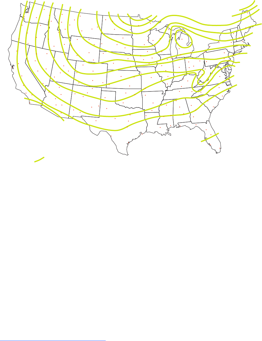
Figure 13. Extreme depth of frost map.
0.49
0.82
1.64
2.46
3.28
4.10
4.92
5.74
5.74
4.92
4.10
3.28
3.28
2.46
1.64
0.82
0.49
0
0
0
0
4.10
7.38
7.38
7.38
7.38
8.20
8.20
8.20
8.20
6.56
6.56
EXPLANATION
Line of equal depth
of possible frozen
soil during winter
Modified from Floyd (1978).
CARIBOU
AUGUSTA
CONCORD
BOSTON
NEW YORK
PHILADELPHIA
WASHINGTON
NORFOLK
ROANOKE
RALEIGH
WILMINGTON
COLUMBIA
ATLANTA
ALBANY
MACON
MIAMI
FT MEYERS
ORLANDO
GAINSVILLE
TALLAHASSEE
PENSACOLA
BILOXI
MERIDIAN
OXFORD
EL DORADO
LITTLE ROCK
FAYETTEVILLE
SPRINGFIELD
COLUMBIA
OTTUMWA
CEDAR
RAPIDS
MASON
CITY
MANKATO
DULUTH
BEMIDJI
DEVILS
LAKE
FARGO
MINOT
WILLISTON
GLENDIVE
HAVRE
MILES CITY
BILLINGS
GREAT
FALLS
HELENA
BUTTE
SALMON
LEWISTON
SPOKANE
OMAK
MISSOULA
KALISPELL
MINNEAPOLIS
DES MOINES
FORT
DODGE
JACKSON
BATON
ROUGE
CORPUS
CHRISTI
GALVESTON
SHREVEPORT
DEL RIO
AUSTIN
WACO
DALLAS
LAWTON
TULSA
WICHITA
TOPEKA
ST JOSEPH
ENID
HAYS
LINCOLN
NORFOLK
MITCHELL
PIERRE
ABERDEEN
BISMARK
LEAD
NORTH PLATTE
CHADRON
CHEYENNE
CASPER
GILLETTE
SHERIDAN
CODY
JACKSON
ROCK SPRINGS
DODGE CITY
LAMAR
DENVER
CRAIG
PUEBLO
GRAND
JUNCTION
DURANGO
ABILENE
PECOS
TUCSON
MIAMI
PHOENIX
PRESCOTT
FLAGSTAFF
KINGMAN
LAS VEGAS
ELY
AUSTIN
RENO
REDDING
LAKEVIEW
LONGVIEW
YAKIMA
SEATTLE
BEND
SALEM
BURNS
BAKER
PENDLETON
MEDFORD
ELKO
WINNEMUCCA
TONOPAH
GRAND CANYON
CEDAR CITY
SAN DIEGO
LOS
ANGELES
BAKERSFIELD
SAN FRANCISCO
SACRAMENTO
FRESNO
SAN
BERNARDINO
GREEN
RIVER
IDAHO
FALLS
TWIN
FALLS
BOISE
PROVO
LOGAN
RICHFIELD
LAS CURCES
ROSWELL
PORTALES
ALBUQUERQUE
GALLUP
SANTA FE
RATON
SILVER
CITY
LUBBOCK
AMARILLO
MONTGOMERY
BIRMINGHAM
FLORENCE
NASHVILLE
KNOXVILLE
LOUIS VILLE
DAYTON
COLUMBUS
CANTON
LIMA
KALAMAZOO
DETROIT
GRAND
RAPIDS
GRAYLING
MARQUETTE
WAUSAU
ELY
EAU CLAIRE
LA CROSSE
MADISON
CHICAGO
AURORA
PEORIA
DECATUR
MT VERNON
MARION
INDIANAPOLIS
BOWLING GREEN
LEXINGTON
CHARLESTON
ASHEVILLE
RICHMOND
ALBANY
SYRACUSE
BUFFALO
MONTPIELIER
SCRANTON
READING
ERIE
PITTSBURGH
CLARKSBURG
CLARKSBURG
CHARLESTON
Frequency of Gaging-Station Levels 17
Frequency of Gaging-Station Levels
Gaging-station locations and environments vary widely
as do the factors affecting the stability of reference marks and
gages. The relative stability of a gaging station needs to be
considered when determining the frequency at which levels
should be run. For example, a station affected by ground
freezing and thawing may require levels to be run annually
in the spring, while a station with gages and reference
marks xed to bedrock that has demonstrated stability may
require levels to be run only every 5 years. Gaging-station
levels should be run frequently enough to capture any gage
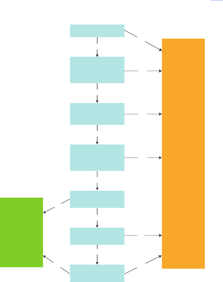
movement that may occur. A decision tree is provided (g. 14)
to help determine when levels need to be run at a gaging
station.
Are there unresolved gage
reading differences?
Has stability at the station
been demonstrated and
documented (see table 5)?
Did the level run from last year
show that the primary reference
gage elevation differs from the
gage datum enough to
require a correction?
Have more than 3 years passed
since the last complete set
of levels were run?
Are less than 3 sets of
annual levels associated with
the current reference gage?
Has an event occurred that
may have disturbed the gaging
station (flood, construction,
vandalism, other)?
Have more than 5 years passed
since the last complete set
of levels were run?
Run levels
Levels are
not needed
YES
YES
YES
YES
YES
YES
YES
NO
NO
NO
NO
NO
NO
NO
IP021599_Figure 14. Decision tree
Figure 14. Decision tree for determining if levels are needed.
18 Levels at Gaging Stations
In addition to running levels according to the site-
specic determined frequency, levels should be run whenever
a difference in gage readings cannot be resolved or damage
is suspected. Suspected damage to a gage may be associated
with ooding, ice, vandalism, nearby construction, or other
events that may disturb some part of the gaging station. A new
gage installation (including the installation of a new reference
gage at an existing station) should have three sets of annual
levels, including the initial establishment set, acquired during
the rst 3 years of operation. After the rst three sets of levels
are acquired, a level frequency of once every 3 years may be
adopted. A level frequency of at least every 5 years may be
adopted if stability is shown to exist. Stability is demonstrated
if the maximum elevation difference from the initial elevations
for the primary reference gage and three reference marks is
less than |0.015| ft for a minimum of ve sets of levels and a
period of at least 10 years (table 5). This means that for any
set of levels run during a 10-year period, the elevations for
the primary reference gage and the three reference marks
(these must be the same three marks measured over the
minimum ve consecutive sets of levels) cannot differ from
the initial elevation (as determined at the beginning of that
10-year period) by |0.015| ft or more. If elevations for any
of these four objective points change by |0.015| ft or more,
the site is not considered stable and the frequency that levels
are run cannot exceed 3 years. An example of a summary of
levels for a station where the stability criterion was not met
is shown in table 6. If during any level run, regardless of the
determined frequency of levels, the elevation of the primary
reference gage differs from the gage datum by |0.015| ft or
more (requiring the gage to be reset and the recorded and
(or) observed stage values to be corrected), levels must be
run again the following year. If no correction is required the
following year, the level frequency can be reset to a 3-year
cycle, until stability can be demonstrated.
Preparation for Running Levels
Running levels at gaging stations is important for
accurate measurements of stage and subsequent computation
of streamow over the life of the station. Uncertainties related
to measurement error during the leveling process can be
minimized if adequate preparations are made. Equipment
should be properly tested and calibrated, and site-specic
information important to the leveling process should be
gathered. Crews assigned to run levels should be properly
trained in the procedures explained in this manual and be
familiar with the equipment they will be using. Levels should
be run in favorable weather conditions and site- specic
environmental conditions; safety hazards that may be
encountered should be understood and discussed before
traveling to the site.
Determining the Need for Levels
The rst step in preparing to run levels is to determine
whether or not levels are needed at a specic gaging station.
The need for levels should be assessed using the decision
tree (g. 14) at least once a year for each station and more
frequently if differences in gage readings cannot be resolved
or damage to the gage is suspected. Ofces are encouraged to
implement a tracking system to determine when levels are due
to be run at each of their stations. It is benecial operationally
Minimum years that a reference gage and three
reference marks have been active
10
Minimum number of sets of levels 5
Maximum difference in elevation from the initial
elevation (as determined at the beginning of a
10-year time period), in feet, of a reference gage
and three reference marks
<|0.015|
Table 5. Requirements for demonstrating gaging station stability.
Date
Elevations
Differences in elevation
Remarks
Reference gage
RM1
(given) RM2 RM3
Water
surface
found
Water
surface
left
Adj.
made
RM1
(given) RM2 RM3
04/01/1999 12.525 8.623 10.226 4.234 4.234 NA NA NA NA
04/14/2000 12.525 8.621 10.228 4.325 4.325 0 0 –0.002 0.002
03/28/2001 12.525 8.622 10.224 3.999 3.999 0 0 –0.001 –0.002
04/02/2004 12.525 8.635 10.242 4.177 4.177 0 0 0.012 0.016 RM3 different by 0.016 ft
04/15/2007 12.525 8.635 10.240 4.440 4.440 0 0 0.012 0.014
04/02/2010 12.525 8.635 10.244 4.013 4.013 0 0 0.012 0.018 RM3 different by 0.018 ft
Table 6. Example summary of levels where the stability criterion is not met.
[All values are given in feet. Elevations are referenced to an arbitrary gage datum. RM, reference mark; adj., adjustment; NA, not applicable; ft, foot]
Running Levels 19
for an ofce to schedule level runs for about one-third of its
stations each year. This will ensure that the leveling workload
in an ofce is balanced and will allow additional stations
that have an immediate need for levels to be run to be more
readily incorporated. The time of year that levels are run at
stations should follow the likely factors that cause changes
to the reference gage. For example, if stations are susceptible
to frost heave, it is best to run levels as soon as possible after
the spring thaw, ideally at temperatures near the standard
temperature of the leveling rod-scale material (usually 68°F).
Compiling Historic Level Notes and Site Sketch
Maps
Past level notes for the station where levels are to be
run should be reviewed. These notes show the previous
composition of the level circuit(s), which can assist in
planning the new level circuit(s). The past level notes can be
used to determine the maximum elevation difference between
the origin and any point in the circuit (L in equation 3).
This information is needed to determine whether or not
the leveling-rod scale must be corrected for expansion or
contraction. The historic level summary should be examined
for any stability issues related to reference marks and
reference points. Finally, copies of the past set of level notes
and the site sketch map should be made and taken to the site.
Considerations for Site Conditions
The expected environmental conditions at the site where
levels are to be run should be considered. The river stage
should be amenable to determining accurate water-surface
elevations from the low water bank and taking FSs to all
reference marks, reference points, and gages. Levels should
be run in favorable weather conditions; wind, rain, and
snow should be avoided if at all possible. Air temperature
and its affect on leveling-rod scales needs to be considered.
Vegetation located in sightlines is undesirable and may be
avoided through maintenance or running levels during times
when leaves are off trees and shrubs. The survey crew should
be briefed on all safety hazards specic to the site where the
levels are to be run. These hazards should be documented and
available in the site-specic job hazard analysis document.
Running Levels
After determining that levels are needed at a gaging
station and making the necessary preparations, levels should
be run following the procedures outlined below. Ideally, the
leveling instrument should be set up in a location that allows
for balanced sightline distances to the objects to be shot from
this instrument setup. The instrument should be placed upon
a rmly set tripod in a stable location at a height that allows
for a comfortable position for the instrument operator and
accurate readings of the rod on the objects to be shot. The
instrument should be properly leveled using the leveling
tools of the instrument. Before beginning the level run, the
time should be noted and all of the gages and recorders at the
station should be read. The temperature of the leveling rod
should be equilibrated to the air temperature. Rod-scale and
air temperatures should be measured and noted. The rod- scale
temperature can be measured directly using an infrared
thermistor, or if the rod is not in the direct sun, air temperature
can be used for the rod-scale temperature. Equation 3 should
be used to determine the maximum expansion or contraction
correction for the level circuit. For this determination, L in
equation 3 should be set equal to the maximum elevation
difference expected between the origin and either the highest
or the lowest point to be surveyed. If the absolute value of the
correction for expansion or contraction due to temperature
variation is greater than 0.003 ft, all FSs and BSs of the level
circuit should be corrected using equation 4.
To describe the procedures for running levels at a gaging
station, a very simple level circuit with two instrument
setups is presented here. Determine the order in which the
reference marks, reference points, gages, water surface, and
other objects are to be shot. The initial instrument height
is determined from a BS to the origin, as determined from
historical levels at the station. The BS value, measured to
the nearest 0.001 ft, should be corrected for expansion or
contraction of the rod scale if needed and then added to the
given elevation of the origin reference mark to obtain the
instrument height. Foresights read to the nearest 0.001 ft
should then be taken to the reference marks, reference points,
gages, water surface, and other objects that were planned
to be shot from the current instrument setup. If appropriate,
FSs should be corrected for temperature-related expansion or
contraction of the rod scale. The corrected FS values should be
subtracted from the corresponding instrument height to obtain
elevations in the gage datum. All gages and recorders should
be read and noted with corresponding times just before or
immediately after the FS on the water surface.
After taking a FS on all objective points that were
planned to be shot from the current instrument setup, a turning
point should be established. The turning point should be a
stable, independent object that is not an objective point of
the level circuit. This point will be used to establish a new
instrument height from which second elevations will be
determined for the objects previously shot. Take a FS on
the turning point, and if necessary, correct for expansion
or contraction, and then determine its elevation. Following
this FS, the instrument should be moved and re-leveled in
a location that again balances the distances to the objective
points. However, if the sightline distances to the objective
points were unbalanced in the initial instrument location, the
new instrument location should invert the sightline distances
by being set up closer to the objective point that was farthest
from the initial setup. Take a BS to the turning point, and if
required, correct for expansion or contraction of the rod scale
20 Levels at Gaging Stations
and add it to the determined elevation of the turning point to
determine a new instrument height. From this new instrument
height, take FSs to the same objective points, correcting for
expansion or contraction if conditions require it, and obtain
second elevations for each. To close the leveling circuit,
the nal shot should be a FS taken on the origin reference
mark that, if necessary, should be corrected for expansion or
contraction of the rod scale.
If a FS on the water surface cannot be taken directly
using the leveling rod, a measurement using a measuring tape
may be made from a reference point from which two FSs
were taken. The length of the tape up or down measurement
should be as short as possible by measuring from a temporary
or permanent reference point on the low water bank from
which two FSs were taken. Tape downs from a bridge or
similar structure should not be used to obtain the water-surface
elevation during a level run.
The procedure presented above describes a simple gaging
station level circuit in which all FSs to objective points can
be taken from a single instrument setup. To help illustrate the
procedures for running levels at gaging stations, a complete
set of level notes from a level circuit that required only two
instrument setups is shown in gure 15. The turning point
that was used to determine the second instrument height was
not an objective point of the circuit. In order to ensure that
two FSs were taken on each objective point of the circuit, an
independent turning point was required. If an objective point
was used as the turning point in this circuit, that objective
point would not have two FSs taken from two different
instrument heights from which elevations could be compared.
Quite often, level circuits are more complex than the one
presented above and require multiple instrument setups, and
thus more than one turning point, to be able to take two FSs
on all objective points. Intermediate turning points, those used
to carry elevations to different instrument setup locations on
either the “out” or the “back” parts of the level circuit, can
be objective points if, when the circuit is completed, they
have two FSs taken on them. Because these objective points
are being used as turning points, they will also have at least
one BS taken on them as well. However, regardless of circuit
complexity, the turning point ascertained after determining
all rst elevations and before determining second elevations
must be independent (not one of the objective points). This
independent turning point marks the termination of the out
part and the beginning of the back part of the level circuit, or
loop. To help illustrate the procedures for running levels at
gaging stations using multiple turning points, a complete set of
level notes from a level circuit that required eight instrument
setups is provided in gure 16. A level notes form, available
for printing and downloading, is provided in appendix C.
Standards and Requirements for Gaging-Station
Levels
Three orders of vertical control classication are accepted
by the Federal Geodetic Control Committee (1984). In
this classication scheme, rst- and second-order leveling
can be applied to the vertical control for National geodetic
surveys, and second- and third-order leveling can be applied
to engineering projects of varying size and scope. Selected
requirements associated with the three classications that
are pertinent to gaging-station levels are presented in table 7.
Gaging-station levels generally are classied as third-
order levels with the adoption of some rst- and second-
order requirements. Table 8 shows adopted standards and
requirements for gaging-station levels.
Circuit-Closure Error
The closure error of a leveling circuit is the difference
between the given elevation for the origin reference mark
and the elevation for that reference mark associated with the
nal instrument height of the level circuit. Closure error is
computed as the given elevation minus the nal elevation.
Assigned vertical closure-error limits dene the desired
and acceptable accuracy, or error, for the intended use of
the survey data. The random acquisition of error in a level
circuit tends to vary with the square root of the number of
opportunities or instrument setups (Davis and others, 1966).
Therefore, a vertical closure-error limit for differential levels
can be determined by multiplying an acceptable uncertainty
constant by the square root of the total number of setups. This
acceptable uncertainty depends on how the data will be used
and should be amenable to the desired accuracy and precision
requirements of the levels. For gaging-station levels, the
uncertainty constant is 0.003 ft (Kennedy, 1990). The vertical
closure-error limit for gaging station level circuits is computed
using the equation
limit
limit
0.003 ,
where
is the closure-error limit, in feet, and
is the total number of instrument
setups in a level circuit.
CE n
CE
n
=
(5)

Running Levels 21
Figure 15. Complete set of level notes for a level circuit with two instrument setups.
System type(s) circle: optical digital
Party
(inst.) (rod)
INSTRUMENT
Make/Model:
Serial Number:
Collimation (optical):
Average of d
2
and d
4
should be less than 110 ft
Collimation test date:
dR
Collimation (digital):
1
Collimation test date:
2
ROD
3
Scale material: ______ CTE ___________ 1/F° or 1/C°
CTE conversions: (1/°F * 1.8 = 1/°C) and ((1/°C)/1.8 = 1/°F)
4
Temperature (T): Rod:___ °F or °C; Air:___ °F or °C
dR
Standard temp (T
o
):
68°F or 20°C or other: ____
1
Given/Origin elevation: _________
2
Max elevation of objective point: ________
3
Min elevation of objective point: _______
c = _______________ft/100ft
c = _______________ft/100ft
as found
as found
4
Max elevation difference (L): _____
ADJUSTMENT (level remains set up at 2 and sighted at R
4
)
C
t
= CTE * L(T-T
o
) C
t
= ________
_
Other devices used as rod (list):
Repeat collimation test
after adjustment
Adjust cross hair to:
Time WS Ref.
Rod taped (circle): yes no
NOTES or SKETCHES:
Rod level used (circle): yes no
GAGE RESET
Ref.
Found
Left
WEATHER:
NOTES:
Circuit
No.
No. of
Inst.
Setups
(N)
Allowable
closure
0.003 *
(N)^.5
Closure
Error
(CE)
CE/N
(take to
0.0001)
CLOSURE ERROR COMPUTATIONS
Computed by: Checked by: Date:
SUMMARY OF OBJECTIVE POINTS
Object
Diff. (1
st
Elev.
-
2
nd
Elev.)
Final Elev.
(Ave. of
Adj. Elev.)
GAGE READINGS
Station Name
Date
Station Number:
U.S. DEPARTMENT OF THE INTERIOR
U.S. Geological Survey
Gaging Station Level Notes
R
1
R
3
R
2
R
4
d
1
d
2
d
3
d
4
1
2
Collimation = c = 100 *
( R
1
+ R
3
)
-
( R
2
+ R
4
)
( d
2
+ d
4
)
-
( d
1
+ d
3
)
c = 100 *
( 4.930 + 5.415 )
-
( 5.772 + 4.572 )
(
137.5 + 73.5 )
-
( 10 + 74 )
c = 100 *
( + )
-
( + )
( + )
-
( + )
PEG TEST OF ENGINEER'S LEVEL
Make/Model:
OPTICAL SYSTEM
DIGITAL SYSTEM
Adj. 1
st
Elev.
Adj. 2
nd
Elev.
IP021599_Fig15_Simple notes_FB
Strawberry River at Pinnacles near Fruitland, Utah
April 20, 2009
MLF RJE
RM2 Given 4.160
4.930 10 RM1 2.788 2.785 0.003 2.786
5.772 137.5 RM4 6.200 6.197 0.003 6.198
5.415 74 CSG 3.820 3.821
-
0.001 3.820
Invar 0.8*10^-6
0.0008
4.572
73.5
OG
2.552 2.548 0.004 2.550
75 75
4.160
6.200
1.520
3.157
<0.0001
none
DCP
OG
OG
13:05 1.52
13:15 1.517 1.52
13:25 1.515 1.52
DCP
13:30 1.52
1.52
1.52
1.52
1.52 1.52 1.52
1.52 1.52
1 2 0.0042
-
0.003
-
0.0015 Clear, sunny, warm
No changes needed or made.
MLF
RJE
April 22, 2009
Leitz Sokkisha Optical
354635
April 20,2009
0.0008
09285900
22 Levels at Gaging Stations
CORRECTED CORRECTED
BS FS
BS+(CTE*
BS*(T
-
T
0
))
FS+(CTE*
FS*(T
-
T
0
))
CLOSURE-
ERROR
ADJUSTMENT
TO HI
ADJUSTED
1
st
ELEVATION
ADJUSTED
2
nd
ELEVATION
OLD
ELEVATION
Remarks
ELEVATION
Remarks
OBJECT BS FSHEIGHT
OF
INSTRU-
MENT
(HI)
FINAL
ELEVATION
DIFFERENCE
(AE1
-
AE2)
5.017
8.335
9.177
6.388
4.160
2.788
6.200
2.788
6.200
3.820
2.552
2.786
4.160
6.198
3.820 3.822
2.550 2.550
1.516
1.512
2.548
3.821
6.197
2.785
2.789
6.201
3.821
2.553
1.517
0.982
2.976
5.356
6.624
7.660
8.195
7.802
6.766
5.493
3.117
6.529
5.154
1.515
2.551
3.824
6.200
2.788
4.163
9.317
RM2
RM1
RM4
CSG
OG
@13:15
@13:25
WS
TP1
Moved Instrument
TP1
WS
OG
CSG
RM4
RM1
RM2
CLOSURE ERROR = 4.160 - 4.163 = -0.003
CElimit = |0.003*(√2setups)| = |0.004|
Given; Cap 15' NE gage
Cap in concrete pier
Bolt in tree 10' SE gage
Index top lower cap
Nail at 2.55
Given, Origin
Ref. gage (staff plate)
Held on rock, +/-.01
OG=1.52, DCP=1.52
Held on rock, +/-.01
Nail at 2.55
OG=1.52, DCP=1.52
-
0.0015
-
0.0030
-
0.001
0.003
0.003
0.004
IP021599_Figure 15 Simple notes_IS
Figure 15. Continued.
Running Levels 23
Figure 16. Complete set of level notes for a level circuit with eight instrument setups.
System type(s) circle: optical digital
Party
(inst.) (rod)
INSTRUMENT
Make/Model:
Serial Number:
Collimation (optical):
Average of d
2
and d
4
should be less than 110 ft
Collimation test date:
dR
Collimation (digital):
1
Collimation test date:
2
ROD
3
Scale material: ______ CTE ___________ 1/F° or 1/C°
CTE conversions: (1/°F * 1.8 = 1/°C) and ((1/°C)/1.8 = 1/°F)
4
Temperature (T): Rod:___ °F or °C; Air:___ °F or °C
dR
Standard temp (T
o
):
68°F or 20°C or other: ____
1
Given/Origin elevation: _________
2
Max elevation of objective point: ________
3
Min elevation of objective point: _______
c = _______________ft/100ft as found
c = _______________ft/100ft as found
4
Max elevation difference (L):_________
ADJUSTMENT (level remains set up at 2 and sighted at R
4
)
C
t
= CTE * L(T-T
o
) C
t
= ________
_
Other devices used as rod (list):
Repeat collimation test
after adjustment
Adjust cross hair to:
Time WS Ref.
Rod taped (circle): yes no
NOTES or SKETCHES:
Rod level used (circle): yes no
GAGE RESET
Ref.
Found
Left
WEATHER:
NOTES:
Circuit
No.
No. of
Inst.
Setups
(N)
Allowable
closure
0.003 *
(N)^.5
Closure
Error
(CE)
CE/N
(take to
0.0001)
CLOSURE ERROR COMPUTATIONS
Computed by: Checked by: Date:
SUMMARY OF OBJECTIVE POINTS
Object
Diff. (1
st
Elev.
-
2
nd
Elev.)
Final Elev.
(Ave. of
Adj. Elev.)
GAGE READINGS
Station Name
Date
Station Number:
U.S. DEPARTMENT OF THE INTERIOR
U.S. Geological Survey
Gaging Station Level Notes
R
1
R
3
R
2
R
4
d
1
d
2
d
3
d
4
1
2
Collimation = c = 100 *
( R
1
+ R
3
)
-
( R
2
+ R
4
)
( d
2
+ d
4
)
-
( d
1
+ d
3
)
c = 100 *
( 4.834 + 4.715 )
-
( 2.643 + 6.901 )
( 109.4 + 108.9 )
-
( 9.6 + 10.2 )
( 4.940 + 4.559 )
-
( 2.748 + 6.747 )
( 109.1 + 108.7 )
-
( 9.9 + 10.2 )
c = 100 *
PEG TEST OF ENGINEER'S LEVEL
Make/Model:
OPTICAL SYSTEM
DIGITAL SYSTEM
Adj. 1
st
Elev.
Adj. 2
nd
Elev.
IP021599_Fig16_Simple notes_FB
Green River near Jensen, Utah
April 19, 2009 MLF TAK
15.410
25.685
16.290
26.471
25.688
16.290
26.472
-
0.003
-
0.001
0.000
25.686
16.290
26.472
GivenRM1
RM3
RM4
ChkBar
Fiberglass
20*10^-6
0.0025
6.901
108.9
4.715
10.2
2.643
109.4
4.834
9.6
--
70
70
4.940 9.9
15.410
2.748 109.1
26.472
4.559 10.2
3.114
0.002
6.747 108.7
12.296
<0.0005
none
DCP WW
WW DCP
12:05
12:30
3.11 3.11
3.11 3.11
1 8 0.008
-
0.004 Clear, sunny, warm
No changes needed or made.
TopCon DL-102C
1202
09261000
MLF TAK April 22, 2009
April 19, 2009
April 19, 2009
0.0025
0.0020
3.113.11
12:55 3.113.11
3.113.113.114
12:35 3.113.113.114
-
0.0005
24 Levels at Gaging Stations
CORRECTED CORRECTED
BS FS
BS+(CTE*
BS*(T
-
T
0
))
FS+(CTE*
FS*(T
-
T
0
))
CLOSURE-
ERROR
ADJUSTMENT
TO HI
ADJUSTED
1
st
ELEVATION
ADJUSTED
2
nd
ELEVATION
OLD
ELEVATION
Remarks
ELEVATION
Remarks
OBJECT BS FSHEIGHT
OF
INSTRU-
MENT
(HI)
FINAL
ELEVATION
DIFFERENCE
(AE1
-
AE2)
15.410
16.29016.29016.290
16.290
10.026
15.410
25.685
25.688
26.471
25.686
26.472
25.690
26.470
26.472
9.963
3.113
3.112
0.000
-
0.0005
-
0.0010
-
0.003
-
0.001
-
0.0020
-
0.0040
-
0.0025
-
0.0035
-
0.0030
-
0.0015
15.410
3.111
1.552
4.616
9.880
8.670
5.069
2.417
1.682
18.521
9.964
10.028
10.109
18.292
25.464
28.590
28.692
21.344
RM1
16.2912.230RM4
8.412TP1
9WW
3.1146.850
@12:30
@12:35
WS
5.4124.552TP2
3.1146.914
WS
10.028
0
0
WW
8.4121.616TP1
16.2922.000RM4
16.7941.498TP3
23.5211.943TP4
25.6882.902RM3
26.4742.116CHKBR
26.275
26.475
2.315TP5
2.217CHKBR
25.6913.001RM3
19.6629.030TP6
15.4145.930RM1
Closure Error is (15.410-15.414) =
-
0.004
Acceptable closure is 0.003*√8 = |0.008| ft
Brass cap rt. Anchor block
Top of bolt d/s leg A-frame
screwdriver
Direct read
+/
-
0.02
Dial =9.96
Given, Origin
Dial =10.03
Direct read
WW(ref) = 3.11, DCP=3.11
WW(ref) = 3.11, DCP=3.11
+/
-
0.02
Brass cap us right brdg abut
Dial = 26.47
Dial = 26.47
.964
IP021599_Figure 16 Comp notes_IS
Figure 16. Continued.
Running Levels 25
Order First Second Third
Class I II I II
Recommended uses Basic framework of the National
Network and metropolitan
area control. Regional crustal
movement studies. Extensive
engineering projects. Support for
subsidiary surveys.
Secondary frame-
work of the
National Network
and metropolitan
area control. Local
crustal movement
studies. Large
engineering
projects. Tidal
boundary refer-
ence. Support
for lower order
surveys.
Densication within
the National
Network. Rapid
subsidence studies.
Local engineering
projects.
Topographic
mapping.
Small-scale
topographic
mapping.
Establishing
gradients in
mountainous areas.
Small engineering
projects. May
or may not be
adjusted to the
National Network.
Maximum collimation error
(ft/100 ft)
0.005 0.005 0.005 0.005 0.01
Maximum time interval (days)
between collimation error
determinations
1 1 1 1 7
Rod level verticality maintained
to within (ft)
10 10 10 10 10
Maximum sight length (ft) 164 197 197 230 295
Minimum ground clearance of
line of sight (ft)
1.6 1.6 1.6 1.6 1.6
Maximum circuit misclosure
(circuit-closure error limit) (ft)
|0.010√D| |0.013√D| |0.020√D| |0.026√D| |0.039√D|
Table 7. Standards and select requirements for leveling.
[Modied from Federal Geodetic Control Committee (1984) and McCormac (1983). D is distance in kilometers. ft, foot]
Adopted
standards and
requirments
Order Third
Use
Gaging station
levels
Maximum collimation error (ft/100 ft) |0.003|
Maximum time interval (days) between
collimation error determinations
7
Rod level verticality maintained to within (ft) 10
Maximum sight length (ft) 164
Minimum ground clearance of line of sight (ft) 1.6
Maximum circuit misclosure (circuit-closure
error limit) (ft)
|0.003√n|
Table 8. Standards and adopted requirements for gaging station
levels.
[n is the total number of instrument setups in a circuit. ft, foot]
Assessing a Level Circuit and Adjusting
Elevations
An acceptable set of gaging-station levels has two FSs,
each from a different instrument height, to a minimum of
two independent reference marks, all reference points, all
gages, and the water surface. A third independent reference
mark is the origin, or starting point, with a given elevation
from which the initial instrument height is determined. The
origin reference mark is considered to be the most stable and
should be explicitly identied as such in the current station
description for the gaging station. The rst criterion for a valid
level circuit is that the absolute value of the closure error for
the leveling circuit must be less than or equal to the closure
error limit computed using equation 5 and must not exceed
|0.015| ft regardless of the number of instrument setups. If the
closure error exceeds the closure error limit, the entire level
circuit must be re-run.
26 Levels at Gaging Stations
Following the completion of a level circuit for which
the closure error falls within the specied limit, elevations of
objective points are adjusted by distributing the determined
closure error of the circuit to each instrument setup. Closure
error is associated with instrument setups made throughout
a leveling circuit and instrument (collimation) error if
present and sightline distances are not balanced. Closure
error is introduced into a circuit during the determination of
instrument heights because of errors in FS readings taken
on the turning points, or errors in BS readings taken on the
turning points or origin. Closure error is not affected by side
shots, shots taken on objective points from a given instrument
setup. In the levels methods and techniques presented in
this manual, the specic instrument setup(s) where error is
incurred cannot be determined; therefore, closure error is
distributed in a manner that assumes the error accumulates
with each instrument setup. The methods described by Thomas
and Jackson (1981) should be used to adjust the elevations
of objective points by distributing the circuit closure error
uniformly to the different instrument setups of the level
circuit. To determine adjusted elevations for any objective
point in a circuit, use the equation
[( )( / )] ,
w
here
is the adjusted elevation of an objective
point,
is the sequential instrument setup
number associated with the
foresight taken to that objective
point (the fir
adj seq unadj
adj
seq
E HI CE n E
E
HI
= +
st instrument setup is 1,
second instrument setup is 2),
is the closure error for the circuit
computed as the given origin
elevation minus the final elevation
of the origin from the final
instrument s
CE
etup,
is the total number of instrument setups
in the circuit, and
is the unadjusted elevation of the
objective point.
unadj
n
E
(6)
Table 9 gives an example of a four-instrument setup level
circuit where a closure error of -0.005 ft is distributed to the
four instrument setups and the applied error is accumulated
with the sequence of instrument setups. The absolute value of
the closure error of the circuit, 0.005 ft, is less than the closure
error limit, |0.006| ft, computed using equation 5. The closure
error of -0.005 ft shows that the nal elevation of the origin
reference mark was 0.005 ft higher than the given elevation.
The adjustment, calculated by dividing the closure error by the
number of instrument setups and multiplying by the sequential
instrument setup number should be rounded to a precision of
0.0001 ft. This adjustment should be added to the unadjusted
elevations to obtain adjusted elevations that should then be
rounded to a precision of 0.001 ft. Rounding should follow the
technique shown in table 10 (U.S. Geological Survey, 1991).
The closure-error criterion of a valid level circuit
discussed above ensures that systematic errors associated with
instrument setups are not introduced into a leveling circuit.
The second criterion of a valid level circuit is that the absolute
value of the difference between the adjusted rst and second
elevations for each objective point must be less than or equal
to 0.005 ft. This criterion, based on the examination of side
shots, ensures that systematic errors specic to each objective
point are not present in their nal elevations. If the absolute
value of the difference between the adjusted rst and second
elevations for an objective point is greater than 0.005 ft, two
new FSs, each from independent instrument heights, must
be taken. A new closure error for this abbreviated circuit
is determined, and the closure error must fall within the
previously specied tolerance. The new elevations of the
objective points are adjusted, as described above, and the
absolute value of the difference between the adjusted rst and
second elevations must be less than or equal to 0.005 ft.
Elevations for some objects are determined by sighting
them in at the cross hair of the level, such as the bottom of a
wire weight or an electric tape gage weight. When running
levels to these types of objects, they are either lowered or
raised until they are at the cross hair of the level. Therefore,
determined elevations, which are equal to the instrument
height, vary from one instrument setup to another. For this
reason, these types of objects are not subject to the elevation
difference criterion. Although it may be possible to compare
the difference between the height of the instrument and the
dial reading for the 2 FSs, the 0.01 ft precision of the gages
prohibits a comparison that can be held to the |0.005| ft
tolerance. Because taking precise FSs on the water surface is
often difcult, water-surface elevations are not subject to the
|0.005| ft elevation difference criterion as long as uncertainties
in the water-surface measurements are noted (for example,
Sequential
instrument
setup
Amount to add
to initial elevations
(foot)
1 –0.0012
2 –0.0025
3 –0.0038
4 –0.0050
Table 9. Computed adjustment values for each instrument setup
of a four-instrument level circuit with a closure error of –0.005
foot.
[Closure error of circuit: –0.005 foot. The nal elevation of the origin
reference mark was 0.005 foot higher than the given elevation]
Running Levels 27
± 0.01). Final elevations for objective points are calculated
by averaging the adjusted rst and second elevations. The
elevation for the origin reference mark is still the given value.
To properly determine whether a gage needs to be reset, and
if it is reset, to ensure that it is reset correctly, levels must
be computed and checked in the eld. The level note form
provided in appendix C adheres to the gaging-station levels
procedures and requirements presented here.
Methods for Taking Foresights on Gages and the
Water Surface
Two FSs must be taken to all gages and the water surface
from two different instrument heights when levels are run at a
gaging station. Levels are run at gaging stations to make sure
that all gages are properly set and accurately reporting water-
surface elevation in the gage datum. Therefore, these FSs
are the most important shots taken. When gages do not agree
with the gage datum, the survey crew must accurately reset
the affected gages. Many different types of gages are used at
gaging stations, and various techniques are used to take a FS
on each gage type and the water surface. Some of the more
common techniques for taking a FS on gages and the water
surface are presented below.
Vertical Staff Gage
Vertical staff gages are perhaps the type of gage most
commonly found at gaging stations. Staff gages are placed
in direct contact with the water. They can be placed inside
stilling wells or attached to various objects on the banks of a
stream. Stations on streams that have a large range in stage
often have a series of staff plates that are installed in vertical
intervals along a sloping bank. While it is feasible to directly
read staff plates using an engineer’s level, this technique is
usually not practical. The most common method for taking a
FS on a staff plate is to establish a reference point by partially
driving a nail or screw into the staff plate backing next to the
plate. The elevation of the reference point, in relation to the
staff plate, should be read from the plate and noted. To take the
FS, a rod should be held level on the reference point (g. 17).
For the staff plate to agree with the gage datum, the elevation
of the reference point, read using the plate, should equal the
elevation computed from the FS. Staff gages consisting of
multiple plate sections should have a FS taken on all sections
or a measuring tape can be used to measure from a location
where the FSs have been taken on one plate section, such as a
reference point, to each of the other plate sections. For obvious
reasons, staff plates must be installed vertically. A carpenter’s
level should be used to verify that plates are vertical when
levels are run.
Electric Tape Gage
Electric tape gages (ETG) are used in stilling wells to
safely measure the water surface inside the well without
entering the conned space. Electric tape gages are
permanently mounted on a shelf inside the stilling well.
These gages consist of a spooled graduated steel tape with an
attached weight and an analog voltage readout (g. 18). The
gage is connected to a battery terminal, and a lead wire from
another battery terminal is extended below the water surface in
the well. To obtain a gage reading, the ETG weight is spooled
down to the water, and when the bottom of the weight contacts
the water surface, the circuit is closed and the voltage dial
responds. The graduated tape is read at a reading index, called
the ETG index, marked by a line and located just above the
surface on which it is mounted.
Example Original number Rounded number
1 0.32891 0.329 If the rst of the discarded digits is greater than 5, add 1 to the digit representing the
third signicant gure
2 47,543 47,500 If the rst of the discarded digits is less than 5, leave the digit representing the third
signicant gure unchanged
3 11.65 11.6 If the rst of the discarded digits is 5, all the following digits are zero, and the digit
representing the third signicant gure is even, leave the digit unchanged.
4 22.75 22.8 If the rst of the discarded digits is 5, all the following digits are zero, and the digit
representing the third signicant gure is odd, round the digit up to the next even
number.
5 18.05 18.0 If the rst of the discarded digits is 5, all the following digits are zero, and the digit
representing the third signicant gure is zero, leave the digit unchanged.
6 18.051 18.1 If the 5 is followed by any of the digits 1 through 9, add 1 to the digit representing the
third signicant gure
Table 10. Technique for rounding off numbers.
[Modied from Hansen (1991)]
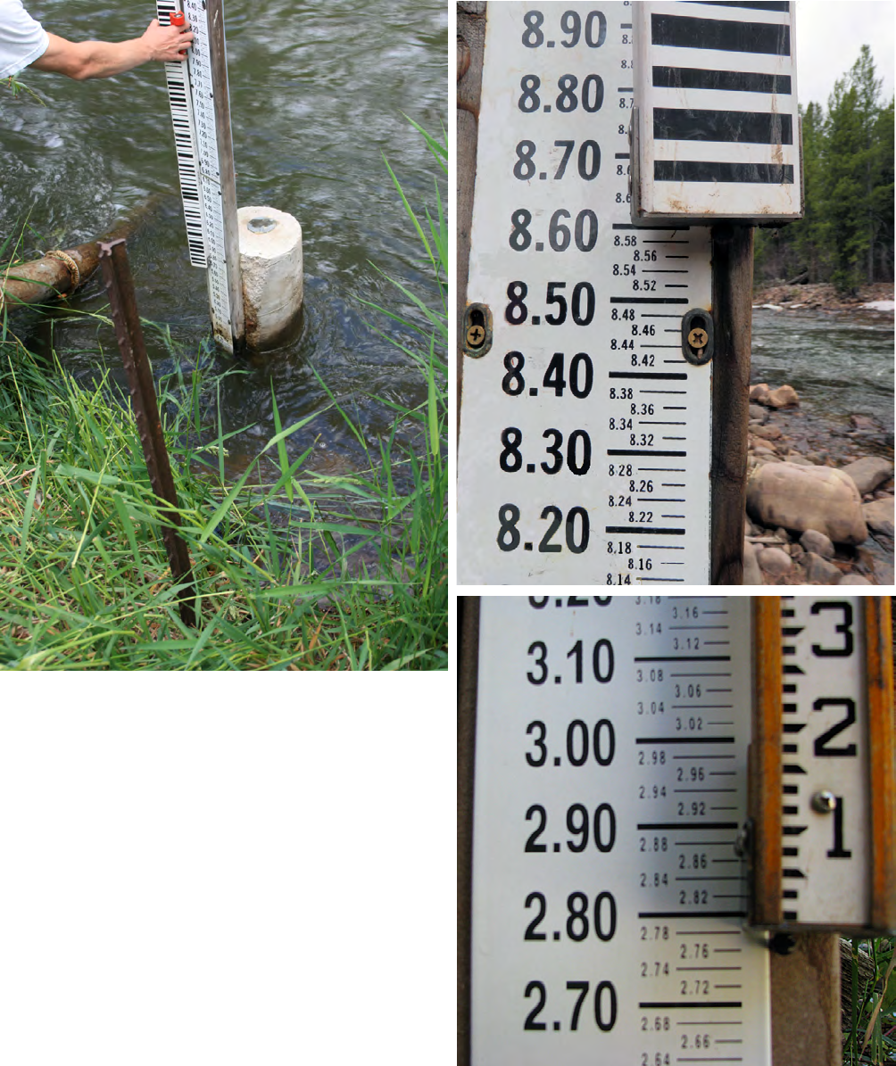
28 Levels at Gaging Stations
Figure 17. Foresights being taken on staff plates
by holding leveling rods on nails driven into backing
boards.
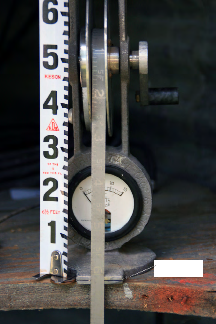
Running Levels 29
Figure 18. Electric tape gage with a pocket rod held on a stack of coins at the elevation of
the index.
IP021599_Figure 18. ETC_coins
Electric tape gage
index

30 Levels at Gaging Stations
When running levels at a station with an ETG, FSs
should be taken on the ETG index, and when feasible, FSs
should also be taken on the bottom of the weight. A slight gap
exists between the ETG index and the object on which it is
mounted. When taking a FS on the ETG index, be sure that the
rod, which is likely a carpenter’s ruler, a measuring tape, or a
“pocket rod,” is set at the level of the ETG index. A stack of
coins on the shelf can usually be used as a stable place to hold
the rod and obtain an accurate FS (g. 18).
Foresights taken on the bottom of the ETG weight should
be taken with the weight as close to the water surface as
possible. However, unless the stilling well is equipped with a
clean-out door, the FS on the bottom of the weight will likely
be taken with the weight located just below the instrument
shelf. The level should be set up so that the instrument height
is at least one length of the weight lower than the ETG index.
To take a FS, the ETG weight should be lowered until the
bottom of the weight is at the cross hairs of the level. While
the weight is at this location, the gage height should be read
at the ETG index. If the ETG agrees with the gage datum, the
instrument height will equal the reading at the ETG index.
Electric tape gages are susceptible to any movement of the
shelter they are installed in. They are also sensitive to any
movement of the shelf that they are mounted on. Adding
weight, such as a larger battery, to an instrument shelf may
cause the shelf to ex downwards, which could change the
elevation of the ETG index and cause incorrect gage height
readings.
Wire-Weight Gage
Wire-weight gages are most often installed on bridge
structures (g. 19), but can also be installed on a cantilever on
a stream bank (g. 20). Suspended above the water surface,
wire-weight gages are weighted cables that are spooled on
a calibrated drum. To take a gage reading, the weighted
cable is lowered until the bottom of the weight contacts the
water surface. The gage-height value is read from the digital
counter and the calibrated drum of the wire-weight gage. The
contact with the water surface is determined visually, which
introduces uncertainty associated with the sightline distance,
lighting, and the surface characteristics of the water. When
running levels to a wire-weight gage, a FS should be taken on
both the check bar (g. 19) and the bottom of the weight near
the water surface. For cantilever installations (only), FSs on
the check bar are not required as they are not associated with
the elevation of the weight of the wire-weight gage; however,
tracking elevations of the check bar of a cantilevered wire-
weight gage may be useful in determining stability of the
cantilever structure.
Foresights taken on the check bar of a traditional wire-
weight gage are taken with the check bar in its outer position
(away from the object it is mounted on) using a leveling rod.
Foresights taken on the bottom of the weight for all wire-
weight gages should be taken from an instrument set up on
the low water bank, such that the FS is taken with the wire
weight as close to the water surface as possible. The wire
weight should be lowered until the bottom of the weight is at
the cross hairs of the level. With the weight at this location,
the gage height should be read from the digital counter and
the calibrated drum. If the wire-weight gage agrees with the
gage datum, the instrument height will equal the reading of the
wire-weight gage.
A wire-weight gage has several potential sources of error
to be considered when checking it (Kennedy, 1990). The drum
is calibrated so that every rotation accounts for a distance
traveled by the weight. For this reason, the cable should be
evenly spooled on the drum. Wire weights tend to spin as
they are lowered and raised. If the cable is not allowed time
to unwind, it will be twisted and thus shorter. This can lead
to incorrect gage heights. After the cable reaches its proper
length, the wire weight should be spooled back up onto the
drum. The weight should be placed on the check bar, and the
associated check bar reading should be noted. The weight can
then be lowered to the water surface to determine the gage
height. These procedures should be followed when taking a FS
on the bottom of the weight as well.
Variations in the drum and the cable diameter of a wire-
weight gage can cause calibration errors (Kennedy, 1990).
Gage height readings from a wire-weight gage represent a
count of the number of revolutions made by the calibrated
drum before the weight contacts the water surface. Any
differences between the actual diameters of the drum and
the cable, and the diameters programmed into the revolution
counter will accumulate as the drum revolves. Fortunately,
because of this accumulation, these calibration errors are linear
and can be corrected for once recognized and documented.
At most gaging stations, wire-weight gages should be
set to accurately read low water elevations. If a wire-weight
gage is properly set to read low water elevations, a calibration
error can be recognized if the check bar reading differs from
the check bar elevation determined from levels. By preparing
a graph of the wire-weight gage readings for the bottom of
the weight and the check bar and the elevations from levels,
corrections for gage height readings at different stages can be
determined (g. 21). The equation for this linear relation is
shown in gure 21 and can be used to compute the correction
to the gage reading by inputting the wire-weight reading.
When such corrections are dened, a plot and an equation
similar to these should be prepared and stored at the gaging
station. The sources of error for wire-weight gages discussed
here are usually negligible for wire-weight gages mounted less
than 15 ft above the water, and increase with greater distances
(Kennedy, 1990).

Running Levels 31
Digital
counter
Calibrations
on drum
Drum with
spooled
cable
Check bar
Weight
Figure 19. Wire-weight gages mounted on bridges.
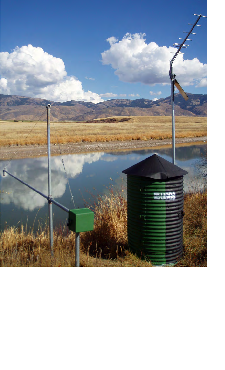
32 Levels at Gaging Stations
Figure 20. Cantilevered wire-weight gage located to the left of a stilling well.
IP021599_Figure 20. Cantilever wire-weight.
Crest-Stage Gage
Crest-stage gages (CSG) record the peak water-surface
elevation, or gage height, as a high water mark consisting
most often of a cork line on a stick inside a pipe. A vertically
installed pipe, which is capped on the top and bottom,
communicates with stream water by a set of holes drilled into
a cap on the bottom of the pipe. As the water-surface elevation
decreases, the maximum level of the water is recorded by a
cork line on a stick contained within the pipe. To recover the
recorded maximum instantaneous gage height, the stick is
removed from the pipe and the distance from the bottom or the
top of the stick to the cork line is measured. If the index of the
CSG is located at the bottom, the stick is measured up from
the bottom. If the index is at the top, the stick is measured
from the top.
Foresights taken on the index of a CSG can usually be
taken with a leveling rod. The location where the leveling rod
is held depends on location of the index. Often, the bottom
cap has a metal stud attached in the center where the stick
rests (g. 22 inset). The elevation of this stud is equal to the
cap surface where the threads begin, and the FS is taken by
holding the rod on the top of the bottom cap (g. 22). A bolt
installed through the pipe near the bottom provides a surface
Running Levels 33
Figure 21. Stage-related wire-weight corrections determined from levels.
Correction value = 0.024 - 0.0024*Wire-weight gage reading
5
0.020.0
-
0.02
-
0.06
-
0.1
-
0.04
-
0.08
10
15
20
25
30
35
40
45
50
IP021599_Figure 21. WW correction
WIRE-WEIGHT GAGE READING, IN FEET
CORRECTION TO WIRE-WEIGHT GAGE READING, IN FEET
46.27 46.182 -0.088
9.89 9.890 0
Object Wire-weight
gage reading,
in feet
Wire-weight
checkbar
Wire-weight
at height of
instrument
Elevation
from levels,
in feet
Correction to
wire-weight gage
reading, in feet
for the stick to rest on and is an excellent index to hold a rod
on to take a FS (g. 23). For both of these CSG congurations,
the maximum stage is determined by measuring from the
bottom of the stick to the cork line high water mark and then
adding that value to the elevation of the CSG index. Some
CSGs have the index on the top of the stick. Foresights are
taken by holding the leveling rod on top of the stick at the
index, and the maximum stage is determined by measuring
from the top of the stick down to the cork line high water mark
and then subtracting that value from the elevation of the CSG
index.
Inclined Staff Gage
Inclined staff gages are permanent structures that are
installed at about the same slope as the streambank (g. 24).
The scale along the incline is set to represent the water-surface
elevation. The slope of these gages minimizes damage caused
by debris and ice. The permanence of the inclined staff gages
makes them very difcult to adjust if they disagree with
the gage datum. Foresights are taken on several foot marks
throughout the gage’s range, from one or more instrument
heights (Kennedy, 1990). If the inclined staff gage is a
composite of multiple slopes, at least 2 FSs must be taken on
each slope.
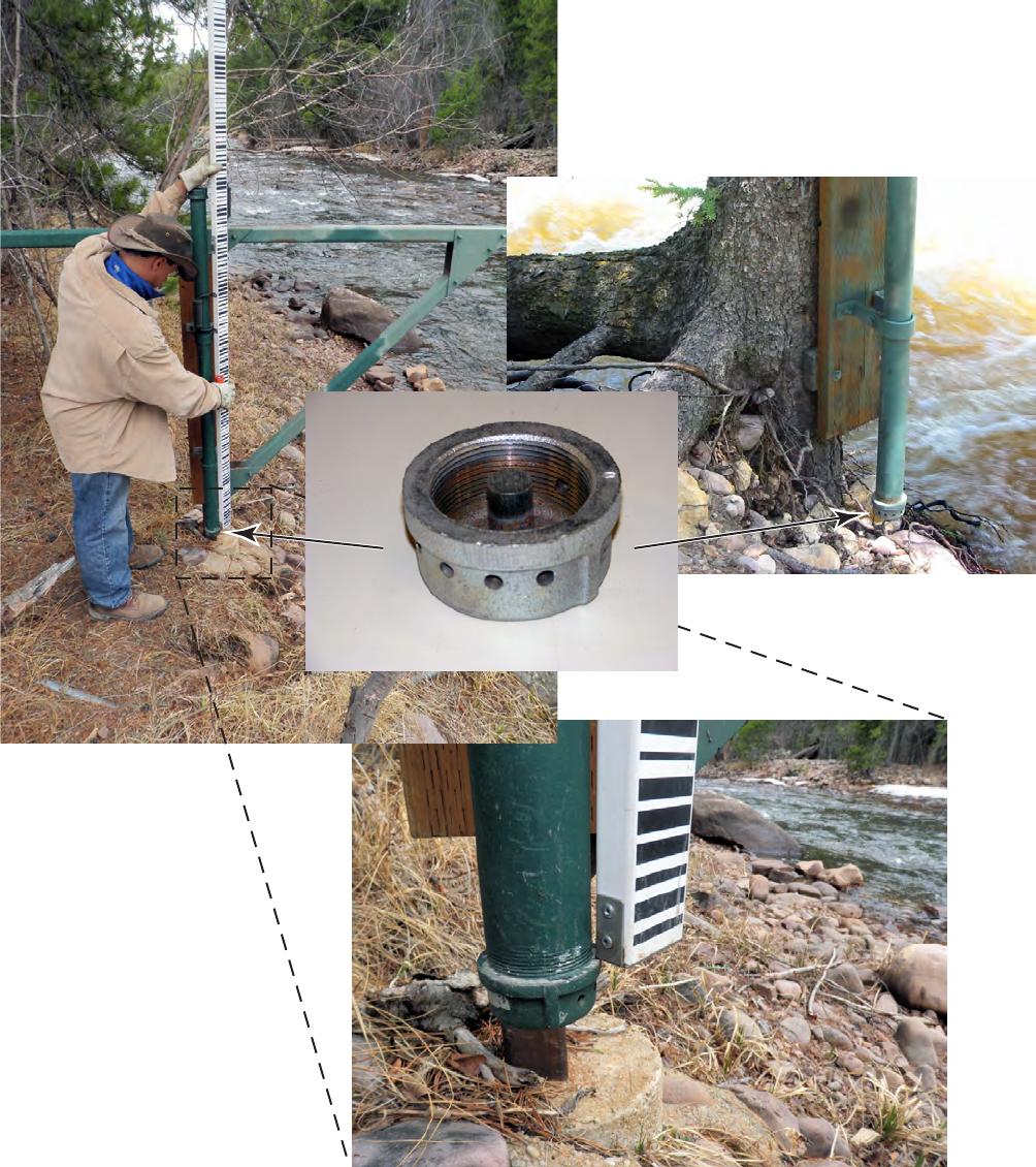
34 Levels at Gaging Stations
Figure 22. Crest-stage gage where the index is the bottom cap. Inset
photograph of the bottom cap showing the internal stud.
IP021599_Figure 22. Rising level auto gages.
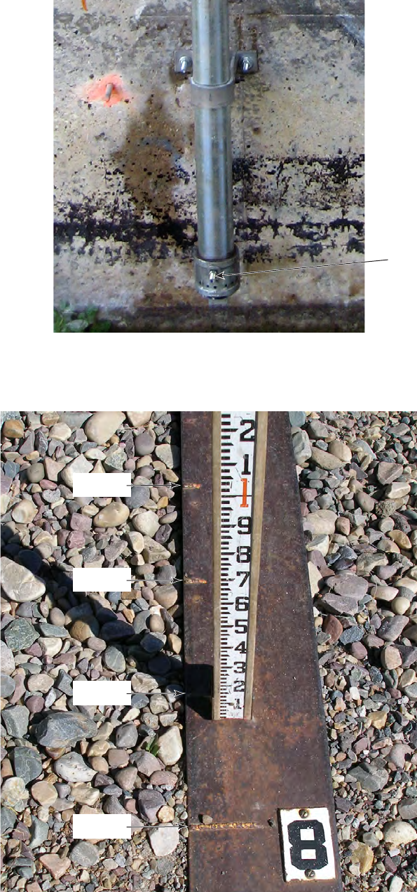
Running Levels 35
Figure 23. Crest-stage gage where the index is a bolt
installed through the pipe.
Figure 24.
Inclined staff gage installed on a streambank.
IP021599_Figure 23. Rising level auto gages.
Bolt
IP021599_Figure 24. Inclined staff rod.
8.30 feet
8.20 feet
8.10 feet
8.00 feet
36 Levels at Gaging Stations
Water Surface
Traditional gaging stations are established to measure the
elevation of the water surface. When running levels at gaging
stations, two FSs are required to be taken on the water surface.
These FSs can be difcult to obtain because the water surface
is not a rm object and therefore a rod cannot be held directly
on it. Also, the water surface may not be vertically stable at
the time and (or) location of the measurement. There are three
techniques that can assist in taking precise and accurate FSs
on the water surface. For streams that are shallow along the
banks, a stable object such as a rock, a stake, or a screwdriver
driven to the water surface, or even the wading boot of the
rod man can be used as a stable location to hold a leveling
rod. These objects will have to be positioned in a manner
that allows a visual determination of the water surface and
rm placement of the bottom of the leveling rod. A second
technique that can be used if stream conditions (including
depth and velocity) allow is to hold the rod on the streambed,
take a FS of the elevation of the streambed, and manually
read the depth of the water off of the rod. To determine the
elevation of the water surface, compute the elevation of
the streambed and add the water depth to it. Finally, if the
conditions of the stream do not allow both of these techniques,
a reference point (either a temporary or a permanent one) can
be established as close as possible to the water surface. From
this reference point, a measuring tape can be used to tape
down to the water surface. An estimate of the uncertainty in
the FS taken on the water surface should always be provided
by the rod man and included in the remarks on the level notes.
Resetting Gages Based on the Results of Levels
The main purpose of running levels at gaging stations is
to verify that gages, specically the primary reference gage,
are properly set to read the stage in the gage datum. The
primary reference gage should be reset if the absolute value of
the difference between the elevation reading of the reference
gage and the gage datum is greater than or equal to 0.015 ft.
Before the gage is reset, the level circuit containing the gage
must be completed. A complete level circuit is one in which
circuit closure error is less than or equal to the established
limit, adjustments associated with closure error have been
applied, differences between the adjusted rst and second
elevations of objective points have been computed, and it
has been veried that these differences meet the established
criteria. Final elevations for all gages are determined and the
computations for the circuit are checked. If the reference gage
needs to be reset, it should be reset on the basis of the nal
computed elevation.
The survey crew must verify and document that the gage
was reset correctly. There are three verication methods: (1)
an abbreviated level circuit consisting of a closed objective
point (part of a completed and valid level circuit), the gage,
and a turning point (2) a tape down from a reference point
that was part of a completed and valid circuit; and (3) an
independent check of the water-surface elevation and gage
reading. Resetting auxiliary gages (those other than the
primary reference gage) also is recommended when the
difference between the elevation reading of the auxiliary gage
and the gage datum is greater than or equal to |0.015| ft.
Methods for Simplifying Complex Level Circuits
Complex level circuits for the purposes of this discussion
are level circuits that require more than two instrument
setups to obtain two independent FSs for all objective points.
In a complex circuit, elevation must be carried from one
instrument setup location to another by using intermediate
turning points to establish more than two instrument heights.
After obtaining all rst FSs and before obtaining second FSs,
an independent turning point that is not an objective point is
required to establish the rst instrument height from which
second FSs will be taken. In contrast, simple level circuits
have only two instrument setups, with the second instrument
height being established from an independent turning point
that is not an objective point to take second FSs.
The error tolerances set forth for circuit closure and for
differences between adjusted rst and second elevations are
strict. The method described by Thomas and Jackson (1981)
for distributing closure error by instrument setup assumes that
error is evenly accumulated through the level circuit. While
this assumption may not always be true, this method provides
the best means available for distributing closure error because
it is difcult, if not impossible, to determine the specic
instrument setups where errors are incurred within a leveling
circuit. Unfortunately, this method of error distribution, and
its underlying assumption, can lead to incorrect adjustments to
valid elevations.
Level circuits with more than two instrument setups
have more opportunity to incur error in both closure and nal
elevations. By limiting the number of instrument setups in a
circuit, the potential for error can be minimized. In most cases,
by implementing some of the techniques discussed below, a
level circuit consisting of more than two instrument setups
can be broken down into a series of independent level circuits,
each having a minimum of two instrument setups.
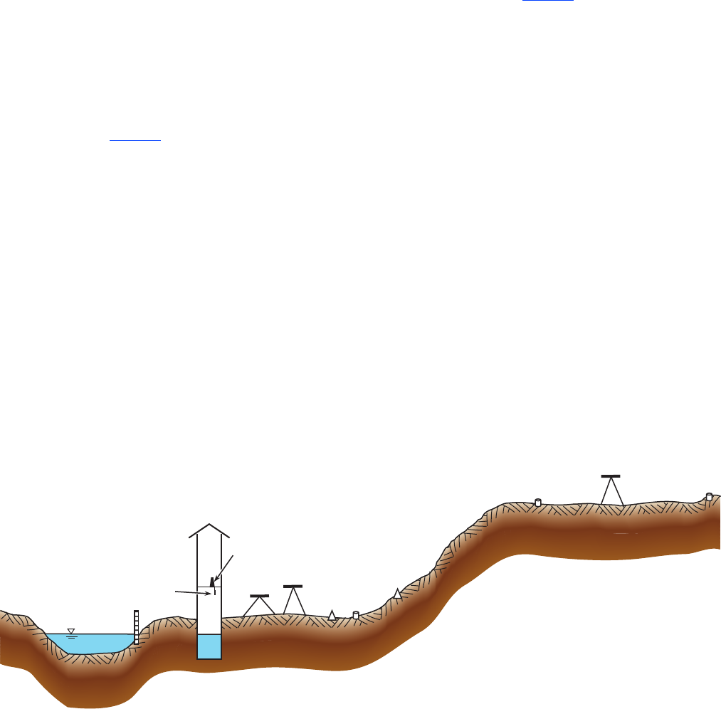
Running Levels 37
Separating Complex Level Circuits into a Set of
Sequentially Closed Simple Level Circuits
Most complex level circuits can be broken down into
a series of simple level circuits that are closed in sequence.
A simple level circuit requires a turning point that is not an
objective point, and a complex level circuit needs to carry
elevation using an objective point(s) or an intermediate turning
point(s), and requires at least one turning point that is not an
objective point.
Level notes and a leveling diagram for a complex level
circuit are shown in gure 25. Shots from a single instrument
setup cannot be taken on all of the objective points of this
circuit: RM1, RM2, RM3, the ETG index, the bottom of the
ETG weight, the outside staff gage, and the water surface.
RM1 (the origin) and RM2 are located up a slope above the
other objective points at the site. This level circuit uses an
intermediate turning point (TP1) to carry elevation down to
the remaining part of the circuit. From the second instrument
setup, FSs are taken on the ETG index, the outside staff
gage, the water surface and RM3. RM3 is then used as an
intermediate turning point to establish the third instrument
height, which is needed to take a FS on the bottom of the ETG
weight. An independent turning point is established (TP2) and
the circuit is shot in reverse order back to RM1.
The complex level circuit described above can be broken
down into three simple level circuits that are sequentially
closed. Level notes and a leveling diagram for the three simple
level circuits are shown in gure 26. The rst simple circuit
consists of objective points RM1, RM2, and TRM1. RM1
is the origin and is used as the starting point to set the initial
instrument height. A temporary reference mark, TRM1, is
established in the rst simple level circuit to carry elevation
to the second circuit. Note that the location of TRM1 is the
same as that of the rst turning point in the complex leveling
circuit diagram discussed above. An independent turning
point (TP1) is established to ensure that two FSs are taken on
each of the objective points for the rst level circuit, which
includes RM2 and TRM1. This rst circuit is closed with the
second FS taken on RM1. The second simple circuit consists
of objective points TRM1, RM3, the ETG index, the outside
staff gage, and the water surface. The initial height of the
instrument for the second circuit is determined from TRM1
which had two FSs taken on it in the rst circuit. The second
instrument height is determined from an independent turning
point (TP2). This circuit is closed with the second FS taken on
TRM1. Finally, the shots to the bottom of the ETG weight are
made from a nal simple circuit in which the initial instrument
height is determined from RM3, which had two FSs taken on
it in the second circuit. The second instrument height for the
third simple circuit is determined from an independent turning
point (TP3), and the circuit is closed with the second FS taken
on RM3
Figure 25. A. Leveling diagram showing objective points in a complex circuit and B. level notes for a complex leveling circuit.
2,5
3,4
1,6
RM3
RM2
RM1
TP1,
TP3
TP2
IP021599_Figure 25a. Complex curcuit
Staff
gage
Gaging
station
Water
Surface
ET
index
EXPLANATION
RM
TP
Reference mark
Turning point
ET
index
ET
weight
1,2
Electric tape index
Electric tape weight
Represents the sequential
instrument setup number
ET
Weight
A
38 Levels at Gaging Stations
DIFFERENCE
(AE1
-
AE2)
CORRECTED CORRECTED
BS FS
BS+(CTE*
BS*(T
-
T
0
))
FS+(CTE*
FS*(T
-
T
0
))
CLOSURE-
ERROR
ADJUSTMENT
TO HI
ADJUSTED
1
st
ELEVATION
ADJUSTED
2
nd
ELEVATION
OLD
ELEVATION
Remarks
ELEVATION
Remarks
OBJECT BS FSHEIGHT
OF
INSTRU-
MENT
(HI)
FINAL
ELEVATION
4.655
17.023
14.144
14.144
12.233
12.300
14.146
17.103
29.499
14.146
30.666 26.011 26.011
25.235
15.470
15.210
15.210
15.470
25.235
26.011
10.340
10.340
12.300
9.550
14.144
25.235 25.235 25.235
15.210
10.340
12.300
15.210
10.340
12.300
15.210
10.340
12.300
9.550
9.550
12.300
14.146
15.210
25.235
10.340
9.550
1.553
1.844
1.846
7.553
6.763
1.893
1.633
4.264
3.488
1.913
14.029
4.803
1.911
1.813
6.683
7.473
4.723
5.431
15.196
RM1
RM2
TP1
Moved Instrument
TP1
0.0000
0.0000
0.0000
0.000
0.000
0.000
0.000
OG
@13:20
@13:30
WS
RM3
Moved Instrument
RM3
TP2
Moved Instrument
TP2
RM3
Moved Instrument
RM3 0.0000
WS
OG
3PT
Moved Instrument
TP3
0.0000
RM2
RM1
CLOSURE ERROR = 26.011- 26.011 = 0.000
+/
-
0.01, DCP = 9.55
+/
-
0.01, DCP = 9.55
ETG (ref)=9.55, OG=9.55
nail @ 10.34
ETG reads 14.15Ref. gage , Direct Read
ETG reads 14.14Ref. gage, Direct Read
Mounted on shelf
Staff, Nail @ 10.34
ETG(ref)=9.55, OG=9.55
Brass cap 12' E
Given, OriginBrass cap upslope 50' E
Brass cap upslope 35' E
CElimit = |0.003*(√6setups)| = |0.007|
0
0
ETG
Index
ETG
Index
ETG
Weight
ETG
Weight
B
Figure 25. Continued.
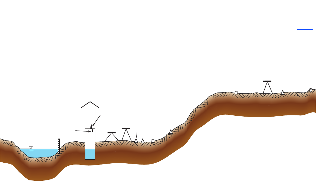
Running Levels 39
3,4
5,6
1,2
RM3
RM2
RM1
TRM1
TP2
Staff
gage
Gaging
station
Water
Surface
ET
index
TP1
TP3
IP021599_Figure 26. Simple circuit
EXPLANATION
RM
TP
TRM
Reference mark
Turning point
Temporary reference mark
ET
index
ET
weight
1,2
Electric tape index
Electric tape weight
Represents the sequential
instrument setup number
ET
Weight
A
Figure 26. A. Leveling diagram and B. level notes showing 3 simple level circuits used to replace 1 complex level circuit.
Both the complex level circuit and the set of three
simple circuits have a total of six instrument setups. A distinct
difference is that in the complex circuit, elevation is carried
through the six instrument setups consecutively, whereas in
the simple circuits, elevation is carried through two setups
at a time. The six setups in the complex circuit represent
six opportunities where errors can occur. We assume that if
present, these errors accumulate and will be represented in the
closure error for the circuit. Where these types of errors occur
within the circuit cannot be determined, and in a case such as
this one, the closure error is distributed evenly to each of the
six instrument setups. In the set of three simple level circuits,
only two instrument setups were needed in each circuit to
take FSs on the objective points and close the circuit. That
created only two locations in each circuit where error could be
introduced. All three simple circuits were closed sequentially,
which ensured that elevations assigned to TRM1 and RM3,
used to determine instrument heights for the second and third
circuits, respectively, were valid before running those circuits.
If an error is introduced into one of the simple circuits, that
error can be recognized and rectied before shooting all
objective points twice at the site. The above examples also
demonstrate that sequentially closing the simple circuits
eliminates the need to go back up the slope to the origin
reference mark, RM1. The accuracy and efciency in running
levels at gaging stations can be improved by breaking down
a complex level circuit into a series of simple level circuits.
Strategic placement of permanent reference marks, such as in
locations where elevation has to be carried up or down a slope,
would reduce the need to establish temporary reference marks
or intermediate turning points for every level run.
Using a Suspended Weighted Steel Tape to Carry
Elevation to or from a Bridge Structure
Many gaging stations are separated by a range in
elevation that is greater than the length of one extended
leveling rod. This often happens when reference marks,
reference points, and (or) the wire- weight gage are located
on a bridge that is relatively high above the stream, and
other reference marks, reference points, various gages, and
the water surface are located well below the bridge deck.
Kennedy (1990) describes how a weighted steel tape can be
suspended from a bridge and be used as a long leveling rod
to carry elevation from a lower streamside level circuit to a
higher level circuit on the bridge deck (and vice versa). This
method incorporates running a series of simple level circuits.
The effects of thermal expansion and contraction, tension,
and wind must be understood and the precision and accuracy
requirements attainable before using a suspended steel tape
for levels (see section on “Leveling Rods”). Two sets of level
notes, one presenting the bridge-down method and the other
the ground-up method, and a leveling diagram are provided as
an example of how to use a suspended weighted steel tape to
run a series of simple level circuits at a gaging station (g. 27).
40 Levels at Gaging Stations
Figure 26. Continued.
CORRECTED CORRECTED
BS FS
BS+(CTE*
BS*(T
-
T
0
))
FS+(CTE*
FS*(T
-
T
0
))
ELEVATION
Remarks
OBJECT BS FSHEIGHT
OF
INSTRU-
MENT
(HI)
DIFFERENCE
(AE1
-
AE2)
CLOSURE-
ERROR
ADJUSTMENT
TO HI
ADJUSTED
1
st
ELEVATION
ADJUSTED
2
nd
ELEVATION
OLD
ELEVATION
Remarks
FINAL
ELEVATION
B
30.666
30.750
26.011 26.011
26.011
25.235
25.235
16.514
25.235
16.514
25.235 25.235
16.514
16.514
25.235
16.514
16.514
16.514
15.210
15.210
10.340
10.340
11.455
16.524
12.300
12.300
12.300
12.300
25.002
4.655
5.431
5.664
5.515
4.739
5.800
2.890
7.760
8.550 9.550
15.210
10.340
12.300
15.210
10.340
12.890
15.210
10.340
12.890
9.550
9.550
15.210
10.340
12.300
9.550
1.576
8.613
7.823
2.953
2.655
1.855
0
0
5.863
1.649
14.152
14.236
18.100
18.163
5.748
RM1
RM2
TRM1
TP1
TP1
Moved Instrument
0.0000
0.0000
0.0000
0.0000
0.0000
0.0000
0.000
0.000
0.000
0.000
0.000
TRM1
RM2
RM1
CE = 26.011-26.011 = 0.000 CElimit =|0.003*(√2setups)|=|0.004|
1.586
1.639
TRM1
RM3
ETG
Index
ETG
Index
ETG
Weight
ETG
Weight
OG
@13:25
@13:30
WS
TP2
TP2
Moved Instrument
Moved Instrument
WS
OG
RM3
TRM1
CE=16.514-16.514=0.000 CElimit=|0.003*(√2setups)|=|0.004|
14.100
14.155
14.155 14.155
14.100 14.100
1.800
2.710
RM3
TP3
TP3
RM3
CE=12.300-12.300=0.000 CElimit=|0.003*(√2setups)|=|0.004|
ETG reads 14.16Ref gage, direct read
ETG reads 14.10
Ref gage, direct read
Given
+/
-
0.01, DCP = 9.55
Nail @ 10.34
ETG(ref) = 9.55, OG=9.55
ETG(ref) = 9.55, OG=9.55
+/
-
0.01, DCP = 9.55
Brass cap 12' E
Given
Staff, Nail @ 10.34
Mounted on shelf
Given, Origin
Brass cap upslope 50' E
Brass cap upslope 35' E
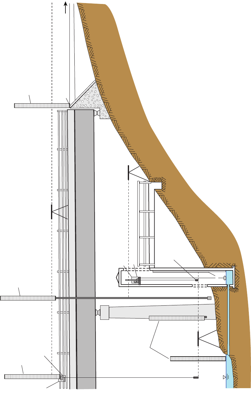
Running Levels 41
Figure 27. A. Leveling diagram and B., C. level notes illustrating the use of a suspended steel tape to carry elevations from a bridge down to a streamside
gage location and from a streamside gage location up to a bridge.
RM1
RM2
RM4
Water
surface
RP1
Electric-tape
gage
Electric-tape
weight
Wire-weight
gage
Check-bar
Suspended steel tape
Index
IP021599_Figure 27a. Suspended tape
Modified from Kennedy (1990).
Leveling rod
Leveling rod
Leveling rod
Leveling rod
EXPLANATION
RM
RP
Reference mark
Reference point
A
42 Levels at Gaging Stations
DIFFERENCE
(AE1
-
AE2)
CORRECTED CORRECTED
BS FS
BS+(CTE*
BS*(T
-
T
0
))
FS+(CTE*
FS*(T
-
T
0
))
CLOSURE-
ERROR
ADJUSTMENT
TO HI
ADJUSTED
1
st
ELEVATION
ADJUSTED
2
nd
ELEVATION
OLD
ELEVATION
Remarks
ELEVATION
Remarks
OBJECT BS FSHEIGHT
OF
INSTRU-
MENT
(HI)
FINAL
ELEVATION
B
3.410
4.302
4.089
3.197
0.873
5.651
8.008
6.909
0
8.142
0
3.365
2.462
0
6.195
1.456
2.328
3.231
0
1.475
1.262
2.895
42.843
42.630
2.682
6.234
6.061
7.043
@10:15
@10:20
46.216 42.806 42.806
42.806
41.914
41.914
20.131
44.741
41.914
44.741
41.914
44.741
44.741
24.909 24.909 24.90924.909
24.909 24.909
3.373
41.914
44.741
3.373
3.373
41.914
44.741
3.373
3.373
3.373
43.321
46.003
22.409 25.782
26.365
22.992
9.434 3.373
7.106
9.434
9.434
6.203
3.373
6.203 6.203
6.203
2.525
9.568
9.568
7.106
3.373
1.426
3.373
9.434
9.434
6.203
1.426
1.426
6.203
9.568
9.568
7.106
1.426
9.568
RM2
RM2
RM1
RM1
RP1
RP1
RM4
RM4
WWCB
WWCB
Tape
Tape
Tape
Tape
Tape
Tape
TP1
CE = 42.806
-
42.806 = 0.000 CElimit = |0.003*(√2setups)|=|0.004|
CE = 3.373
-
3.373 = 0.000 CElimit = |0.003*(√2setups)|=|0.004|
CE = 3.373
-
3.373 = 0.000 CElimit = |0.003*(√2setups)|=|0.004|
0 ft mark on clamped tape is 3.373 ft gage datum
ETG
Index
ETG
Index
ETG
Weight
ETG
Weight
TP2
WS
WW
bottom
WW
bottom
TP3
WS
nail @ 6.20 ft
@ HI
Direct read
Nail @ 6.20 ft
ETG(ref) = 1.43, WW=1.43
@ HI
Moved Inst
@ HI
ETG(ref) = 1.43, WW=1.43
Direct read
Direct read
Bolt E side Rt Pier
@ HI
Direct read
Moved Inst
Clamped @ 40', rod=2.630
Moved Inst
Clamped @ 40', rod=2.843
Brass cap on sidewalk 75'N
Brass cap right abutment
Given, Origin
Check bar reads 44.74
Check bar reads 44.74
Bottom of tape
Given
Given
WW reads 9.43
+/-0.01, DCP=1.43
ETG reads 9.43
ETG reads 9.57
WW reads 9.57
+/-0.01, DCP=1.43
0.0000
0.000
0.000
0.000
0.000
0.000
0.0000
0.0000
0.0000
0.0000
0.0000
Figure 27. Continued.
Running Levels 43
DIFFERENCE
(AE1
-
AE2)
CORRECTED CORRECTED
BS FS
BS+(CTE*
BS*(T
-
T
0
))
FS+(CTE*
FS*(T
-
T
0
))
CLOSURE-
ERROR
ADJUSTMENT
TO HI
ADJUSTED
1
st
ELEVATION
ADJUSTED
2
nd
ELEVATION
OLD
ELEVATION
Remarks
ELEVATION
Remarks
OBJECT BS FSHEIGHT
OF
INSTRU-
MENT
(HI)
FINAL
ELEVATION
2.328
9.434 7.106 7.106
7.106
9.434
6.203
6.203
3.373
3.373
3.373
24.909 24.909 24.909
20.131
24.909
24.909
3.373
1.426
1.426
9.434
9.434
6.203
3.373
6.203
3.373
6.203
1.426
9.434
2.525
9.568
9.568
6.203
3.373
1.426
9.568
9.568
3.231
0
9.568
6.061
6.909
8.008
8.142
0
0
6.195
3.365
2.462
0
7.043
6.234
2.682
5.651
1.456
1.475
3.410
4.302
2.895
4.089
3.197
1.262
42.630
44.741
42.806
41.914
44.741
42.806
41.914
44.741
42.806
41.914
24.909
44.741
42.806
41.914
43.321
41.914
42.806
44.741
41.914
42.806
44.741
3.373
3.373
22.992
0.873
22.409
42.843
26.365
46.216
46.003
25.782
RM1
RM1
ETG
Weight
ETG
Weight
ETG
Index
ETG
Index
RP1
RP1
Tape
Tape
Tape
Tape
Tape
Tape
@ 10:15
@ 10:20
WS
WW
bottom
WW
bottom
TP1
TP2
WS
Bottom of tape = 3.373
WWCB
WWCB
RM2
RM4
TP3
RM4
RM2
Brass cap right abutment
Brass cap on sidewalk 75'N
Clamped @ 40', rod=2.843
Clamped @ 40', rod=2.630
Direct read
Moved Inst
Moved Inst
Direct read
ETG(ref)=1.43, WW=1.43
Direct read
@ HI
nail @ 6.20 ft
Direct read
ETG(ref)=1.43, WW=1.43
@ HI
Moved Inst
@ HI
Bolt E side Rt Pier
@ HI
Given, Origin
WW reads 9.43
ETG reads 9.43
+/
-
0.01, DCP=1.43
Bottom of clamped tape
ETG reads 9.57
WW reads 9.57
+/-0.01, DCP=1.43
Given
Check bar reads 44.74
Given
Check bar reads 44.74
0.0000
0.0000
0.0000
0.0000
0.0000
0.0000
0.000
0.000
0.000
0.000
0.000
0.000
CE = 7.106
-
7.106 = 0.000 CElimit = |0.003*(√2setups)|=|0.004|
CE = 3.373
-
3.373 = 0.000 CElimit = |0.003*(√2setups)|=|0.004|
CE = 3.373
-
3.373 = 0.000 CElimit = |0.003*(√2setups)|=|0.004|
C
Figure 27. Continued.

44 Levels at Gaging Stations
Bridge-Down Method
The diagram in gure 27 shows a weighted steel tape
clamped at its 40.000-ft marking to the bridge deck rail. The
rst level circuit is on the bridge deck and the objective points
are RM2, RM4, the wire-weight check bar, and the clamped
steel tape (noted as “tape” in the level notes). RM2 is the
origin and is used to establish the initial instrument height.
Foresights are taken on the wire-weight check bar and the
bridge deck rail where the tape is clamped. The FS to the top
of the deck rail at the tape is 2.843 ft, noted in the remarks
column in the level notes. The tape is being used as a long
leveling rod; therefore, the FS to the rod at the tape, 2.843 ft,
is added to the suspended length of the tape, 40.000 ft, to
get the representative FS, 42.843 ft. An independent turning
point, TP1, is established and a second instrument height is
determined from which second FSs are taken on the tape,
wire-weight check bar, and RM4. The circuit associated with
the bridge deck is completed by taking a second FS on the
origin, RM2. The rst and second elevations of the 0.000-ft
mark on the suspended tape are determined by subtracting the
representative FSs for the tape from the instrument height.
Both representative FSs for the tape are used to determine that
the elevation at the 0.000-ft mark on the suspended tape is
3.373 ft. The closure error for this circuit is 0.000 ft, elevations
do not need to be adjusted, and the differences between
rst and second elevations for all of the objective points are
0.000 ft.
A second level circuit is about half the distance from the
bridge deck to the low-water bank, and the objective points
are the tape and the ETG index. The instrument height is
established with a BS taken on the tape, which is a direct read
of 22.409 ft. This BS is added to the determined elevation
for the 0.000-ft mark of the tape, 3.373 ft, to determine an
instrument height of 25.782 ft. A FS is taken on the ETG
index and an independent turning point, TP2, is established
to determine the second instrument height. A second FS is
taken on the ETG index and this circuit is completed by taking
a second FS on the suspended tape, which again is a direct
read of the tape. This circuit has a closure error of 0.000 ft,
elevations do not need to be adjusted, and the difference
between rst and second elevations for the ET index is
0.000 ft.
The nal level circuit is on the low-water bank and the
objective points are the tape, RM1, the bottom of the electric
tape weight (ETG weight), RP1, the water surface, and the
bottom of the wire weight (noted as “WW bottom” in the level
notes). Again, the instrument height is established with a BS
taken on the tape, which is a direct read of 6.061 ft. This BS is
added to the determined elevation for the 0.000-ft mark of the
tape, 3.373 ft, to determine an instrument height of 9.434 ft.
From this instrument height, rst FSs are taken on RM1, the
ETG weight through the cleanout door, RP1, the water surface,
and the bottom of the wire weight near the water surface. An
independent turning point is established, TP3, to determine the
second instrument height from which second FSs are taken.
This nal circuit is completed by taking a second FS on the
suspended tape. This circuit has a closure error of 0.000 ft,
elevations do not need to be adjusted, and differences between
rst and second elevations for each of the objective points are
0.000 ft. By using a weighted suspended steel tape clamped
to the bridge deck rail to carry elevation from the bridge
down to the low-water bank, levels can be run at a gaging
station with an elevation difference of over 35 vertical ft using
three sequentially closed level circuits that have a total of six
instrument setups and three turning points.
Ground-Up Method
The ground-up method reverses the procedure for the
bridge-down method and begins from the low-water bank.
A weighted steel tape is clamped at its 40.000-ft marking to
the bridge deck rail. The rst level circuit is on the low-water
bank and the objective points are RM1, the bottom of the
electric tape weight (ETG weight), RP1, the steel tape, the
water surface, and the bottom of the wire weight. The initial
instrument height is established with a BS taken on RM1.
Foresights are taken on the ETG weight through the cleanout
door, RP1, the steel tape, the water surface, and the bottom
of the wire weight near the water surface. An independent
turning point is established, TP1, to determine the second
instrument height from which second FSs are taken on the
objective points. The circuit is completed by taking a nal FS
on the origin, RM1. The elevation of the 0.000-ft mark on the
suspended tape is determined by subtracting the FSs for the
tape from the associated instrument heights. Both FSs taken
on the tape determined that the elevation of the 0.000-ft mark
on the suspended tape is 3.373 ft. The closure error of this
circuit is 0.000 ft, elevations do not need to be adjusted, and
the differences between rst and second elevations for all of
the objective points are 0.000 ft.
A second level circuit is about half the distance from the
low-water bank to the bridge deck, and the objective points
are the tape and the ETG index. The instrument height is
established with a BS taken on the tape, which is a direct read
of 22.409 ft. This BS is added to the determined elevation
for the 0.000-ft mark of the tape, 3.373 ft, to determine an
instrument height of 25.782 ft. A FS is taken on the ETG
index and an independent turning point, TP2, is established
to determine the second instrument height. A second FS is
taken on the ETG index and this circuit is completed by taking
a second FS on the suspended tape, which again is a direct
read of the tape. This circuit has a closure error of 0.000 ft,
elevations do not need to be adjusted, and the difference
between rst and second elevations for the ETG index is
0.000 ft.
The nal level circuit is on the bridge deck and the
objective points are the steel tape, wire-weight check bar,
RM2, and RM4. The instrument height is established with a
BS of 2.843 ft, taken on the top of the deck rail at the tape,

Office Procedures 45
and noted in the remarks column in the level notes. The
tape is being used as a long leveling rod; therefore, the BS
to the rod at the tape is added to the suspended length of
the tape, 40.000 ft, to get the representative BS, 42.843 ft.
The determined elevation for the 0.000-ft mark of the tape,
3.373 ft, is added to the BS to determine an instrument
height of 46.216 ft. From this instrument height, rst FSs
are taken on the wire-weight check bar, RM2, and RM4. An
independent turning point, TP3, is established and a second
instrument height is determined from which second FSs are
taken on RM4, RM2, and the wire-weight check bar. The
circuit associated with the bridge deck is completed by taking
a second FS on the deck rail at the tape. The closure error for
this circuit is 0.000 ft, elevations do not need to be adjusted,
and the differences between rst and second elevations for
all of the objective points are 0.000 ft. By using a weighted
suspended steel tape clamped to the bridge deck rail to carry
elevation from the low-water bank to the bridge deck, levels
can be run at a gaging station with an elevation difference of
over 35 vertical ft using three sequentially closed level circuits
that have a total of six instrument setups and three turning
points.
Office Procedures
The task of running levels at gaging stations includes
some important ofce-related activities. A nal check of the
computations made during the level run that were rst checked
in the eld should be made and documented. Following a level
run, any adjustments made to the elevation of the reference
gage need to be applied to the time series record of gage
height and any other affected measurements of the reference
gage. The eld notes, which include digital les, original
hand written documents, and photographs taken during eld
work, should be stored according to ofce specications. The
historical level summary and station description should be
updated to reect the elevations found during the level run.
Finally, if needed, the site sketch should be updated along with
any descriptions of reference marks that may have changed or
been added since the last level run.
Applying Datum Corrections to Gage Height
Time Series
The primary reference gage at a continuously recording
gaging station is used to set the gage height on the data logger
and to determine the representative gage heights for discharge
measurements. If the level run nds that the absolute value of
the difference between the elevation reading of the reference
gage and the gage datum is greater than or equal to 0.015 ft,
the recorded stage record must be corrected. Corrections
of this type are referred to as datum corrections. Similarly,
observed gage height measurements made during the time
period affected by the datum correction should be adjusted
accordingly. The datum correction applied to the time series
of recorded stage values should be applied in a manner that
is consistent with what caused, or was assumed to cause, the
reference gage elevation to be different from the gage datum.
For example, if the reference gage is damaged during a ood,
the datum correction should be applied at the time the damage
occurs and held constant until the time levels are run and the
reference gage is adjusted. If the reference gage is assumed
to have been heaved by frozen ground during the winter, the
datum correction should be held constant back to the winter
period. If the gage remains ice-free during the winter and
it is believed the reference gage was heaved slowly during
the winter, the datum correction may then be prorated back
through the winter period.
Developing a Site-Specific Historical Level
Summary
A historical level summary that contains the nal
elevations of all objective points from every level run should
be maintained for all gaging stations. The level summary also
should contain descriptions of all reference marks, reference
points, and gages. Other objects of interest that were shot
during a level run, such as the gage height of zero ow or
the orice line terminus, can also be included in the level
summary. The primary reference gage should be explicitly
noted. The level summary provides a way to track elevations
and thus, vertical stability of all objective points over the life
of the station. The stage that each of the various gages at the
station was found to be reading at the beginning of a level run
should be noted as well as the stage each gage was reading at
the end of a level run. The origin reference mark for each of
the level runs should be noted. The historical level summary
should be updated immediately every time levels are run at
the gaging station. A digital summary le provides the best
means for storage and retrieval and can easily be updated. A
form template for the historical level summary for printing or
download is provided in appendix D.
Developing a Site Sketch Map
A sketch map of the site will help anyone who runs
levels at the station. This is especially true for someone who
is unfamiliar with a particular station. This map should show
the locations of the reference marks, reference points, and all
gages with respect to the gaging station structure and other
prominent objects. The location of the low-water control along
with the direction of ow should be included. Recommended
instrument setup locations that provide ideal shot distances are
useful as well. Site sketch maps are best maintained and stored
in digital format.
46 Levels at Gaging Stations
Auxiliary Data to be Obtained During
Level Runs
Running levels at gaging stations provides an opportunity
to acquire other useful elevation-related information. Fresh
high-water marks, if present, should be surveyed and
compared later to recorded gage heights. A cross section of the
hydraulic control(s) (including section, channel, and bank-full
elevations), surveyed in the gage datum, is easy to obtain and
can aid in developing the stage-discharge rating for the site.
The gage height of zero ow associated with the hydraulic
control that denes the low-water stage-discharge relation can
be easily measured when the instrument is set up to measure
the water-surface elevation during levels. Documenting
the elevation, or gage height, at which ow overtops either
bank can assist the USGS and other agencies during ood
conditions. Determining the minimum elevation of a bridge
or road deck in the gage reach can be very useful during
ood events. Measurements of the elevations of various gage
components, such as the orice line terminus or stilling well
intakes, can assist in determining the gage height at which the
gage is out of communication with the stream. A measurement
of the elevation of the instrument shelf provides an estimate of
the likely maximum gage height the data logger can record. In
short, the efciency with which engineer’s levels can obtain
accurate vertical measurements presents opportunities to
acquire auxiliary data when running levels at gaging stations.
Summary
Levels are run at gaging stations to ensure gages are
accurately set to the established gage datum. Differential
leveling techniques are used to determine elevations for
reference marks, reference points, all gages, and the water
surface to a precision of 0.001 foot (ft). Desired accuracy for
a set of station levels is less than 0.010 ft. Precision describes
the closeness of one measurement to another while accuracy
describes how close a given measurement is to the true value.
The techniques presented in this manual provide guidance on
instruments and methods that ensure gaging-station levels are
run to both a high precision and accuracy.
Levels are run at gaging stations whenever unresolved
gage reading differences are identied, damage is suspected
to have occurred to the station, or according to a frequency
recommended for a given station. Engineer’s levels, optical
levels and electronic digital levels, are commonly used for
running levels at gaging-stations. Collimation tests should
be run at least once during any week that levels are run.
Collimation error for an instrument cannot exceed the
absolute value of 0.003 ft/100 ft. Instruments exceeding
this collimation tolerance should be adjusted, and another
collimation test must be run before it is used for gaging-station
levels. If an instrument fails a collimation test, all levels run
since the prior passing collimation test cannot be used and
must be re-run.
An acceptable set of gaging-station levels consists of a
minimum of two foresights, each from a different instrument
height, to at least two independent reference marks, all
reference points, all gages, and the water surface. The initial
instrument height is determined from a third independent
reference mark, known as the origin, or base reference mark.
The absolute value of the closure error of a leveling circuit
must be less than or equal to
0.003 n
ft, where n is the
total number of instrument setups. The entire level circuit
must be re-run if closure error exceeds this threshold; closure
error may not exceed |0.015| ft, regardless of the number
of instrument setups. Closure error for a leveling circuit is
distributed by instrument setups in a manner that assumes
error accumulates linearly and elevations for objective points
are adjusted accordingly. Absolute differences between the
adjusted rst and second elevations for the objective points
in the circuit must be less than or equal to 0.005 ft. Objective
points with absolute differences between adjusted rst and
second elevations exceeding 0.005 ft require two more
foresights from different instrument heights. Final elevations
of objective points are determined by averaging the valid
adjusted rst and second elevations. Reference gages should
be reset if the absolute value of the difference between the
elevation reading of the reference gage and the gage datum
is greater than or equal to 0.015 ft. A summary of selected
requirements and tolerances for gaging-station levels is
provided in appendix E.
References Cited
Breed, C.B., Hosmer, G.L., and Bone, A.J., 1970, The
principles and practice of surveying—Vol. 1., Elementary
surveying (10
th
ed.): London, Wiley and Sons, 717 p.
Corbett, D.M., and others, 1943, Stream-gaging procedure; a
manual describing methods and practices of the Geological
Survey: U.S. Geological Survey Water-Supply Paper 888,
245 p.
Davis, R.E., Foote, F.S., and Kelly, J.W, 1966, Surveying
theory and practice (5
th
ed.): New York, McGraw-Hill,
1096 p.
Federal Geodetic Control Committee, 1984, Standards and
specications for geodetic control networks: National
Oceanic and Atmospheric Administration, accessed on
March 9, 2010, at http://www.ngs.noaa.gov/FGCS/tech_
pub/1984-stds-specs-geodetic-control-networks.htm

References Cited 47
Floyd, R.P., 1978, Geodetic bench marks: National Oceanic
and Atmospheric Administration Manual, National Ocean
Survey, National Geodetic Survey 1, 52 p., accessed on
March 6, 2010, at http://www.ngs.noaa.gov/PUBS_LIB/
GeodeticBMs/
Hansen, W.R., ed., 1991, Suggestions to authors of the
reports of the United States Geological Survey (7th ed.):
Washington, D.C., U.S. Government Printing Ofce, 289 p.
Kennedy, E.J., 1990, Levels at streamow gaging stations:
U.S. Geological Survey Techniques of Water-Resources
Investigations, book 3, chap. A19, 31 p., available online at
http://pubs.usgs.gov/twri/twri3-A19/pdf/twri_3-A19_a.pdf
McCormac, J.C., 1983, Surveying fundamentals: Englewood
Cliffs, New Jersey, Prentice-Hall, 522 p.
Schomaker, M.C., and Berry, R.M., 1981, Geodetic leveling:
National Oceanic and Atmospheric Administration Manual,
National Ocean Survey, National Geodetic Survey 3,
accessed on March 6, 2010, at http://www.ngs.noaa.gov/
PUBS_LIB/Geodeticleveling_nos_3.pdf
Thomas, N.O., and Jackson, N.M., Jr., 1981, Manual
for leveling at gaging stations in North Carolina: U.S.
Geological Survey Open-File Report 81-1104, 37 p.,
available online at http://pubs.usgs.gov/of/1981/ofr81-1104/
pdf/ofr81-1104.pdf
U.S. Geological Survey, 1980, Ground water: National
handbook of recommended methods for water-data
acquisition: Ofce of Water Data Coordination, 149 p.
48 Levels at Gaging Stations
This page intentionally left blank.
Glossary 49
Glossary
Backsight (BS). The reading on a leveling
rod held on a point of known elevation that is
used to establish a height of an instrument.
Benchmark . A permanent marker with
known survey control of vertical and (or)
horizontal coordinates in an established
geodetic system, such as the North American
Vertical Datum of 1988.
Closure error. The difference between the
elevation of the starting point, or origin, of a
closed level circuit and the elevation of that
same point from the final instrument setup;
computed as the given elevation minus the
final elevation.
Collimation. Agreement of a surveying
instrument’s line of sight with its horizontal
axis.
Collimation error. The deviation or
inclination of a level’s line of sight from
horizontal, often given in a vertical deviation
per horizontal distance such as feet per 100
feet; positive when the line of sight points
downward from the instrument.
Curvature and refraction effect. The
increase in a leveling rod’s reading caused by
the combination of the Earth’s curvature and
atmospheric refraction effects.
Datum. A level surface that represents zero
elevation.
Differential leveling. The determination of
the difference in elevation of two points using
a surveying instrument and a leveling rod.
Elevation. The vertical distance from a
point to the datum.
Engineer’s level. A surveying instrument
consisting of a minimum of a telescopic sight
and a sensitive leveling device to make the
line of sight horizontal.
Optical level. An engineer’s level that
is used to manually read a leveling rod.
Electronic digital level. An engineer’s
level with an automated system that reads
a leveling rod.
Foresight (FS). The reading on a leveling
rod held on a point whose elevation is to be
determined.
Gage datum. The zero elevation reference
surface at a gaging station to which all gages
are set.
Gage height. The elevation of the
water surface at a gaging station, used
interchangeably with stage.
Gage height of zero flow. The gage height
at which streamflow ceases. Associated with
the elevation of the lowest point on the low-
water hydraulic control of a gaging station.
Gaging-station levels. Differential levels
run (that is, carried out) at a gaging station to
define and maintain a constant gage datum for
all gages.
Height of instrument (HI). The elevation
of the horizontal line of sight of a surveying
instrument.
Horizontal. A direction that is perpendicular
to the force of gravity.
Parallax. The relative movement of the
image of a leveling rod with respect to
the cross hairs of a surveying instrument
as the observer’s eye moves, caused by
improper focusing of the objective lens of the
instrument.
Reference mark (RM). A permanent marker,
installed in the ground or on a structure,
whose elevation above a set datum is known.
Used to check and make sure that all gages
and reference points are properly set to gage
datum.
Reference point (RP). Objects, often bolts
or screws that are assigned an elevation in
the gage datum. Used to obtain gage heights
when necessary by measuring their distance to
the water surface.
Stage. The elevation of the water surface
at a gaging station, used interchangeably with
gage height.
Temporary reference mark (TRM). A
temporary point of reference that was treated
as an objective point in a previously closed
level circuit that is used to carry elevations to
other instrument setups.
Turning point (TP). A temporary point of
reference in an open level circuit that is used
to carry elevations to other instrument setups
in the level circuit.
Vertical. The direction of the force of
gravity.
This page intentionally left blank.
50 Levels at Gaging Stations
Appendix A 51
Date: _____________________________________
d
2
should be less than 110 ft.
dR
1
2
dR
1
2
c = _______________ft/100ft as found
c = _______________ft/100ft as found
ADJUSTMENT (level remains set up at ORIGINAL LOCATION)
To adjust level, set R
2
to read R
1
To test collimation after adjustment, set up near other scale and repeat measurements.
System adjusted: optical digital R
1
= ______________
NOTES or COMMENTS:
Collimation = c = 100 *
( R
1
-
R
2
)
( d
2
-
d
1
)
(
-
)
(
-
)
c = 100 *
(
-
)
(
-
)
c = 100 *
(
-
)
(
-
)
c = 100 *
FIXED SCALE COLLIMATION TEST OF ENGINEER'S LEVEL
Tested by: _________________________________
OPTICAL SYSTEM
DIGITAL SYSTEM
Circle system type(s): optical digital
Make/Model:
dR
1
2
IP021599_FigA01_Fixed scale_B
R
1
R
2
d
1
d
2
Fixed scale
Fixed scale
Instrument
R
2
R
1
d
1
d
2
Fixed scale
Fixed scale
Instrument
Appendix A. Fixed-Scale Test Form
52 Levels at Gaging Stations
This page intentionally left blank.
Appendix B 53
Appendix B. Peg Test Form
Circle system type(s): optical digital
Average of d
2
and d
4
should be less than 110 ft.
d
R
1
2
3
4
d
R
1
2
3
c = _______________ft/100ft as found
c = _______________ft/100ft as found
c = _______________ft/100ft as found
4
ADJUSTMENT (level remains set up at 2 and sighted at R
4
)
Repeat collimation test
after adjustment.
Adjust cross hair to
NOTES or COMMENTS:
R
1
R
3
R
2
R
4
d
1
d
2
d
3
d
4
1
2
Collimation = c = 100 *
( R
1
+ R
3
)
-
( R
2
+ R
4
)
( d
2
+ d
4
)
-
( d
1
+ d
3
)
c = 100 *
( + )
-
( + )
( + )
-
( + )
c = 100 *
( + )
-
( + )
( + )
-
( + )
( + )
-
( + )
( + )
-
( + )
c = 100 *
PEG TEST OF ENGINEER'S LEVEL
Make/Model:
Date: ____________________________________
Tested by: ______________________________
OPTICAL SYSTEM
DIGITAL SYSTEM
COLLIMATION TEST AFTER ADJUSTMENT
IP021599_Figure B01 Peg Test
54 Levels at Gaging Stations
This page intentionally left blank.
Appendix C 55
Appendix C. Level Notes Form
(Full-size form [8” x 10”] is available for download at http://pubs.usgs.gov/tm/tm3A19)
Circle system type(s): optical digital
Party
(inst.) (rod)
INSTRUMENT
Make/Model: _______________________
Serial Number: ________________________
Collimation (optical): ___________________
Average of d
2
and d
4
should be less than 110 ft.
Collimation test date: ___________________
dR
Collimation (digital): ___________________
1
Collimation test date: ___________________
2
ROD
3
Scale material: ________ CTE _________ 1/F° or 1/C°
CTE conversions: (1/°F * 1.8 = 1/°C) and ((1/°C)/1.8 = 1/°F)
4
Temperature (T): Rod:_____ °F or °C; Air:_____ °F or °C
dR
Standard temp (T
o
):
68°F or 20°C or other: _______
1
Given/Origin elevation: ______________
2
Max elevation of objective point: ______________
3
Min elevation of objective point: ______________
c = _______________ft/100ft as found
c = _______________ft/100ft as found
4
Max elevation difference (L): _______________
ADJUSTMENT (level remains set up at 2 and sighted at R
4
)
C
t
= CTE * L (T
-
T
o
) C
t
= ____________
_
Other devices used as rod (list):
Repeat collimation test
after adjustment.
Adjust cross hair to
Time WS Ref.
Rod taped (circle): yes no
NOTES or SKETCHES:
Rod level used (circle): yes no
GAGE RESET
Ref.
Found
Left
WEATHER:
NOTES:
Circuit
No.
No. of
Inst.
Setups
(n)
Allowable
closure
0.003 √ n
Closure
Error
(CE)
CE/(n)
(take to
0.0001)
CLOSURE-ERROR COMPUTATIONS
Computed by: Checked by: Date:
SUMMARY OF OBJECTIVE POINTS
Object
Difference
(AE1
-
AE2)
Final
Elevation
((AE1+
AE2)/2)
GAGE READINGS
Station Name
Date
Station Number:
U.S. DEPARTMENT OF THE INTERIOR
U.S. Geological Survey
Gaging Station Level Notes
R
1
R
3
R
2
R
4
d
1
d
2
d
3
d
4
1
2
Collimation = c = 100 *
( R
1
+ R
3
)
-
( R
2
+ R
4
)
( d
2
+ d
4
)
-
( d
1
+ d
3
)
c = 100 *
( + )
-
( + )
(
+ )
-
( + )
c = 100 *
( + )
-
( + )
( + )
-
( + )
PEG TEST OF ENGINEER'S LEVEL
Make/Model:
OPTICAL SYSTEM
DIGITAL SYSTEM
COLLIMATION TEST AFTER ADJUSTMENT
dR
1
2
3
4
c = _______________ft/100ft as found
c = 100 *
( + )
-
( + )
(
+ )
-
( + )
Adjusted
1
st
Elevation
(AE1)
Adjusted
2
nd
Elevation
(AE2)
56 Levels at Gaging Stations
DIFFERENCE
(AE1
-
AE2)
CORRECTED CORRECTED
BS FS
BS+(CTE*
BS*(T
-
T
0
))
FS+(CTE*
FS*(T
-
T
0
))
CLOSURE-
ERROR
ADJUSTMENT
TO HI
ADJUSTED
1
st
ELEVATION
ADJUSTED
2
nd
ELEVATION
OLD
ELEVATION
Remarks
ELEVATION
Remarks
OBJECT BS FSHEIGHT
OF
INSTRU-
MENT
(HI)
FINAL
ELEVATION
Appendix D 57
(Given)
Descriptions of objective points:
RM1 —
RM2 —
RM3 —
RP1 —
RP2 —
RP3 —
CSG Index —
ORIFICE —
REF GAGE —
GZF —
STATION NUMBER
Reference Marks and Reference Points
Primary Reference Gage
DATE PARTY
Wire-weight gageStaff gage
Water
surface
by
levels
Water
surface
found
Water
surface
left
Water
surface
found
Water
surface
left
Check
bar(Aux
wire-
weight)
Orifice
line
terminus
Gage
height of
of zero
flow
Datum
correction Remarks
Btm of
weight
nr water
surface
Check
bar
Electric
tape
index
Index
found
Index
left Found Left
Adjust.
made
Auxillary gage Crest Stage gage Recorder
STATION NAME
Appendix D. Historical Level Summary Form
(Digital Excel format is available for download at http://pubs.usgs.gov/tm/tm3A19)
HISTORICAL LEVEL SUMMARY
58 Levels at Gaging Stations
This page intentionally left blank.

Appendix E 59
[n is the number of instrument setups in level circuit. ft, foot; <, less than; | | , absolute value]
Requirements and tolerances
Precision of gaging station levels 0.001 ft
Accuracy of gaging station levels <0.01 ft
Maximum number of days since the last collimation test 7
Maximum collimation error of level instrument |0.003| ft/100 ft
Maximum allowable difference between rod scale and tape check |0.002| ft
Minimum number of reference marks in a level run 3
Maximum temperature correction, Ct, computed using maximum
vertical distance from origin (equation 3) that does not require
correcting all shots for thermal expansion or contraction
|0.003| ft
Maximum allowable clos ure error |0.003√n| and not to exceed |0.015| ft
Minimum number of foresights to
at least two reference marks 2
all reference points 2
all gages 2
the water surface 2
the origin reference mark 1
Minimum number of non-objective point turning points 1
Maximum allowable difference between the adjusted rst and the
adjusted second elevations of objective points
|0.005| ft
Maximum allowable difference between the elevation reading of the
reference gage and the gage datum
<|0.015| ft
Appendix E. Summary of Selected Requirements and Tolerances for Gaging
Station Levels
60 Levels at Gaging Stations
This page intentionally left blank.
Publishing support provided by the U.S. Geological Survey
Publishing Network, Sacramento and Tacoma Publishing Service Center
For more information concerning the research in this report, contact the
Chief, Office of Surface Water
U.S. Geological Survey
12201 Sunrise Valley Drive
Reston, Virginia 20192
http://water.usgs.gov/osw/
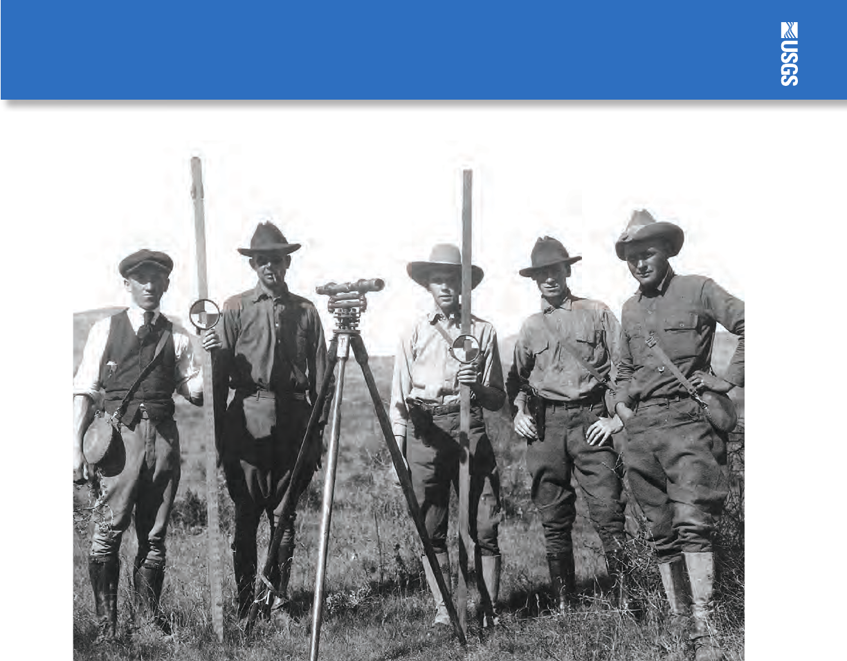
Kenney—Levels at Gaging Stations—Techniques and Methods 3
-
A19
